February 5, 2025
by Olga Filippova
 It has been a while since we wrote on the Elphel Development Blog. However, it doesn’t mean we haven’t been developing new technologies and applications. In fact, there is so much new that I would want to write a post for each new project once it is possible, i.e., after Ukraine wins the war.
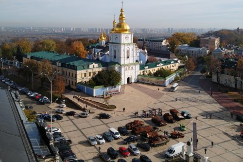
From the beginning of the war, Elphel, Inc. has supported Ukraine against the Russian invasion. We temporarily (until the Victory) painted the Elphel icon in blue and yellow colors of the Ukrainian flag to express our support. In May 2023, Elphel went to Ukraine as part of a Utah Humanitarian and Defense delegation led by the President of the Utah Senate, Mr. Stuart Adams. We represented defense and aerospace companies from our state. During a meeting with the Deputy Minister of the Economy of Ukraine, Mr. Fomenko, he emphasized the country’s priorities in demining for agriculture. Ukraine currently lacks the technology necessary to demine fields in a reasonable amount of time.
This meeting and an idea from Ukrainian engineers at Midgard Dynamics to use the high sensitivity of the Elphel LWIR-16 camera led to developing a game-changing mine-detection system for humanitarian and agricultural needs.
Elphel tested the prototype and presented the results to the scientists from V.M. Glushkov Institute of Cybernetics of NAS of Ukraine. We are currently working with European partners to integrate Elphel technology with humanitarian demining efforts in Ukraine and other countries around the world.
Search and Rescue is another application of this technology.
Here is a link to my recent statement on LinkedIn.
July 16, 2021
by Andrey Filippov and Fyodor Filippov
Advance Steel 2024: https://abcoemstore.com/product/autodesk-advance-steel-2024/ System Requirements Learn about the system requirements for configuring Advance Steel.
Download links for: video and captions.
This research “Long-Range Thermal 3D Perception in Low Contrast Environments” is funded by NASA contract 80NSSC21C0175
June 1, 2020
by Oleg Dzhimiev
Basically, one need to direct the ip cam stream (mjpeg or rtsp) to a virtual v4l2 device which acts like a web cam and is automatically picked up by a web browser or a web cam application. This can be easily done by gstreamer or ffmpeg.
Quick setup
Install and create a virtual webcam
~$ sudo apt install v4l2loopback-dkms

~$ sudo modprobe v4l2loopback devices=1
Direct the stream
The options below are for gstreamer/ffmpeg and rtsp/mjpeg streams:
gstreamer:
# rtsp stream

~$ sudo gst-launch-1.0 rtspsrc location=rtsp://192.168.0.9:554 ! rtpjpegdepay ! jpegdec ! videoconvert ! tee ! v4l2sink device=/dev/video0 sync=false

# mjpeg stream

~$ sudo gst-launch-1.0 souphttpsrc is-live=true location=http://192.168.0.9:2323/mimg ! jpegdec ! videoconvert ! tee ! v4l2sink device=/dev/video0
ffmpeg:
# rtsp stream

~$ sudo ffmpeg -i rtsp://192.168.0.9:554 -fflags nobuffer -pix_fmt yuv420p -f v4l2 /dev/video0

# mjpeg stream

~$ sudo ffmpeg -i http://192.168.0.9:2323/mimg -fflags nobuffer -pix_fmt yuv420p -r 30 -f v4l2 /dev/video0
Finally
Start a video conference application, select the webcam from the menu (/dev/video0).
Test link: meet.jit.si
(more…)
August 4, 2019
by Andrey Filippov
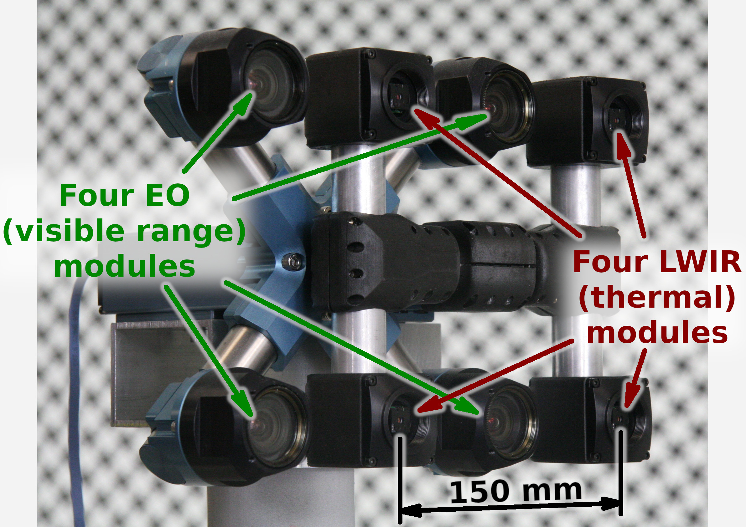
Figure 1. Talon (“instructor/student”) test camera.
Update: arXiv:1911.06975 paper about this project.
Summary
This post concludes the series of 3 publications dedicated to the progress of Elphel five-month project funded by a SBIR contract.
After developing and building the prototype camera shown in Figure 1, constructing the pattern for photogrammetric calibration of the thermal cameras (post1), updating the calibration software and calibrating the camera (post2) we recorded camera image sets and processed them offline to evaluate the result depth maps.
The four of the 5MPix visible range camera modules have over 14 times higher resolution than the Long Wavelength Infrared (LWIR) modules and we used the high resolution depth map as a ground truth for the LWIR modules.
Without machine learning (ML) we received average disparity error of 0.15 pix, trained Deep Neural Network (DNN) reduced the error to 0.077 pix (in both cases errors were calculated after removing 10% outliers, primarily caused by ambiguity on the borders between the foreground and background objects), Table 1 lists this data and provides links to the individual scene results.
For the 160×120 LWIR sensor resolution, 56° horizontal field of view (HFOV) and 150 mm baseline, disparity of one pixel corresponds to 21.4 meters. That means that at 27.8 meters this prototype camera distance error is 10%, proportionally lower for closer ranges. Use of the higher resolution sensors will scale these results – 640×480 and longer baseline of 200 mm (instead of the current 150 mm) will yield 10% accuracy at 150 meters, 56°HFOV.
(more…)
June 18, 2019
by Andrey Filippov
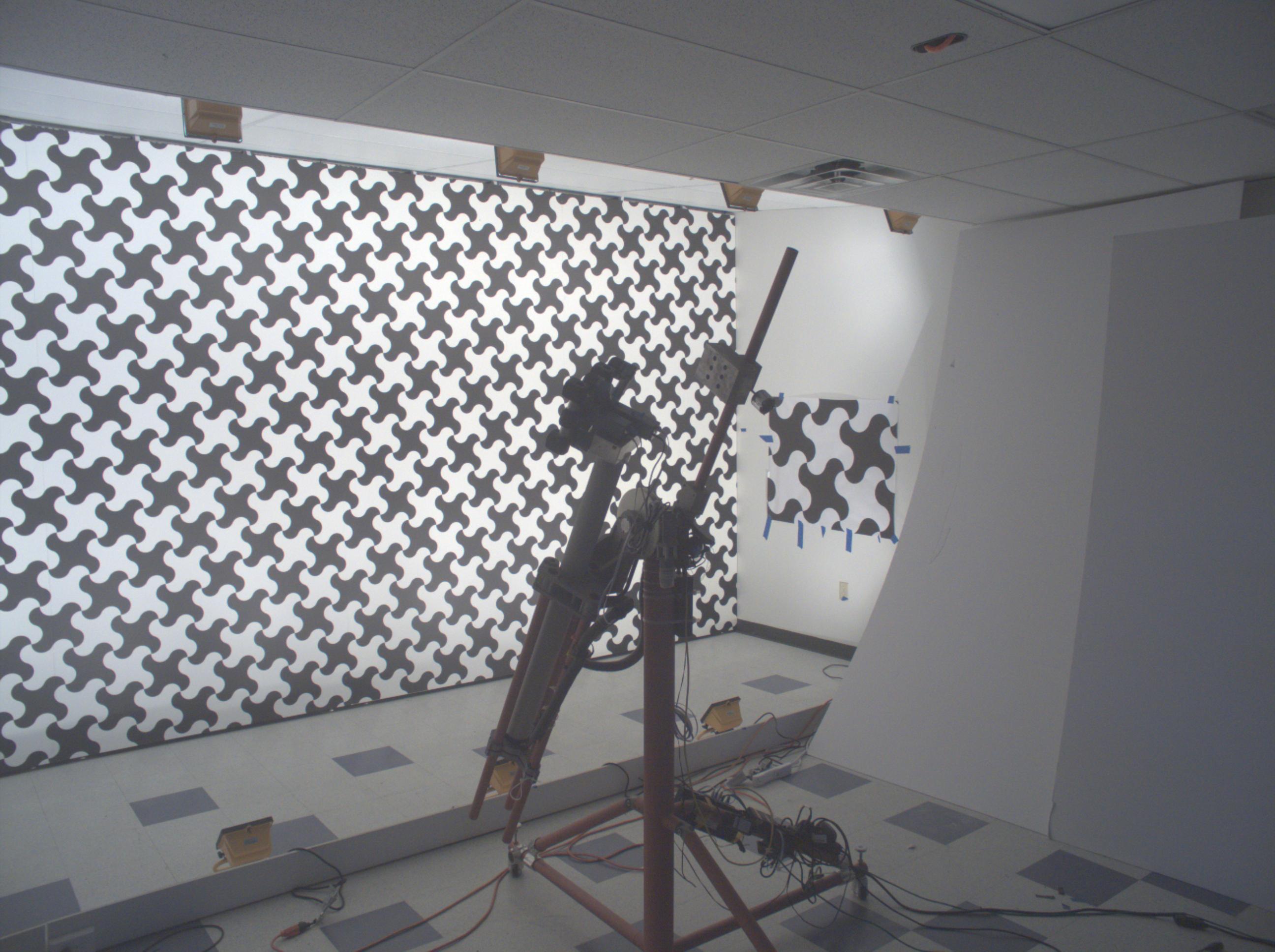
Figure 1. Calibration of the quad visible range + quad LWIR camera.
We’ve got the first results of the photogrammetric calibration of the composite (visible+LWIR) Talon camera described int the previous post and tested the new pattern. In the first experiments with the new software code we’ve got average reprojection error for LWIR of 0.067 pix, while the visible quad camera subsystem was calibrated down to 0.036 pix. In the process of calibration we acquired 3 sequences of 8-frame (4 visible + 4 LWIR) image sets, 60 sets from each of the 3 camera positions: 7.4m from the target on the target center line, and 2 side views from 4.5m from the target and 2.2 m right and left from the center line. From each position camera axis was scanned in the range of ±40° horizontally and ±25° vertically.
(more…)
June 6, 2019
by Andrey Filippov
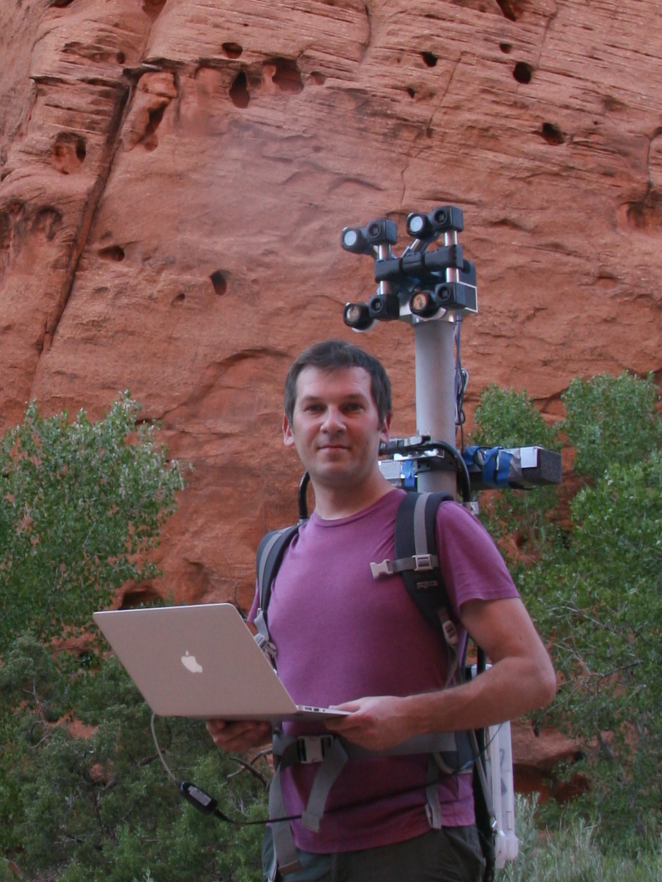
Figure 1. Oleg carrying combined LWIR and visible range camera.
While working on extremely long range 3D visible range cameras we realized that the passive nature of such 3D reconstruction that does not involve flashing lasers or LEDs like LIDARs and Time-of-Flight (ToF) cameras can be especially useful for thermal (a.k.a LWIR – long wave infrared) vision applications. SBIR contract granted at the AF Pitch Day provided initial funding for our research in this area and made it possible.
We are now in the middle of the project and there is a lot of the development ahead, but we have already tested all the hardware and modified our earlier code to capture and detect calibration pattern in the acquired images.
(more…)
October 11, 2018
by Andrey Filippov
After we coupled the Tile Processor (TP) that performs quad camera image conditioning and produces 2D phase correlation in space-invariant form with the neural network[1], the TP remained the bottleneck of the tandem. While the inferred network uses GPU and produces disparity output in 0.5 sec (more than 80% of this time is used for the data transfer), the TP required tens of seconds to run on CPU as a multithreaded Java application. When converted to run on the GPU, similar operation takes just 0.087 seconds for four 5 MPix images, and it is likely possible to optimize the code farther — this is our first experience with Nvidia® CUDA™.
(more…)
September 5, 2018
by Andrey Filippov
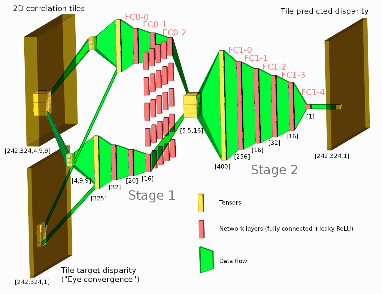
Figure 1. Network diagram. One of the tested configurations is shown.
Neural network connected to the output of the Tile Processor (TP) reduced the disparity error twice from the previously used heuristic algorithms. The TP corrects optical aberrations of the high resolution stereo images, rectifies images, and provides 2D correlation outputs that are space-invariant and so can be efficiently processed with the neural network.
What is unique in this project compared to other ML applications for image-based 3D reconstruction is that we deal with extremely long ranges (and still wide field of view), the disparity error reduction means 0.075 pix standard deviation down from 0.15 pix for 5 MPix images.
See also: arXiv:1811.08032
(more…)
July 21, 2018
by Olga Filippova
In this blog article we will recall the most interesting results of Elphel participation at CVPR 2018 Expo, the conversations we had with visitor’s at the booth, FAQs as well as unusual questions, and what we learned from it. In
addition we will explain our current state of development as well as our near and far goals, and how the exhibition helps to achieve them.
The Expo lasted from June 19-21, and each day had it’s own focus and results, so this article is organized chronologically.
Day One: The best show ever!
June 19, CVPR 2018, booth 132
While we are standing nervously at our booth, thinking: “Is there going to be any interest? Will people come, will they ask questions?”, the first poster session starts and a wave of visitors floods the exhibition floor. Our first guest at the booth spends 30 minutes, knowledgeably inquiring about Elphel’s long-range 3D technology and leaves his business card, saying that he is very impressed. This was a good start of a very busy day full of technical discussions. CVPR is the
first exhibition we have participated in where we did not have any problems explaining our projects.
The most common questions that were asked:
(more…)
July 20, 2018
by Andrey Filippov
We uploaded an image set with 2D correlation data together with the import Python code for experiments with the neural networks and are now looking for collaboration with those who would love to apply their DL experience to the new kind of input data. More data will follow and we welcome feedback to make this data set more useful.
The application area we are interested in is an extremely long distance 3D scene reconstruction and ranging with the distance to baseline ratio of 1000:1 to 10,000:1 while preserving wide field of view. Earlier post describes aircraft distance and velocity measurements with up to 3,000:1 distance-to-baseline ratio and 60°(H)×45°(V) field of view.
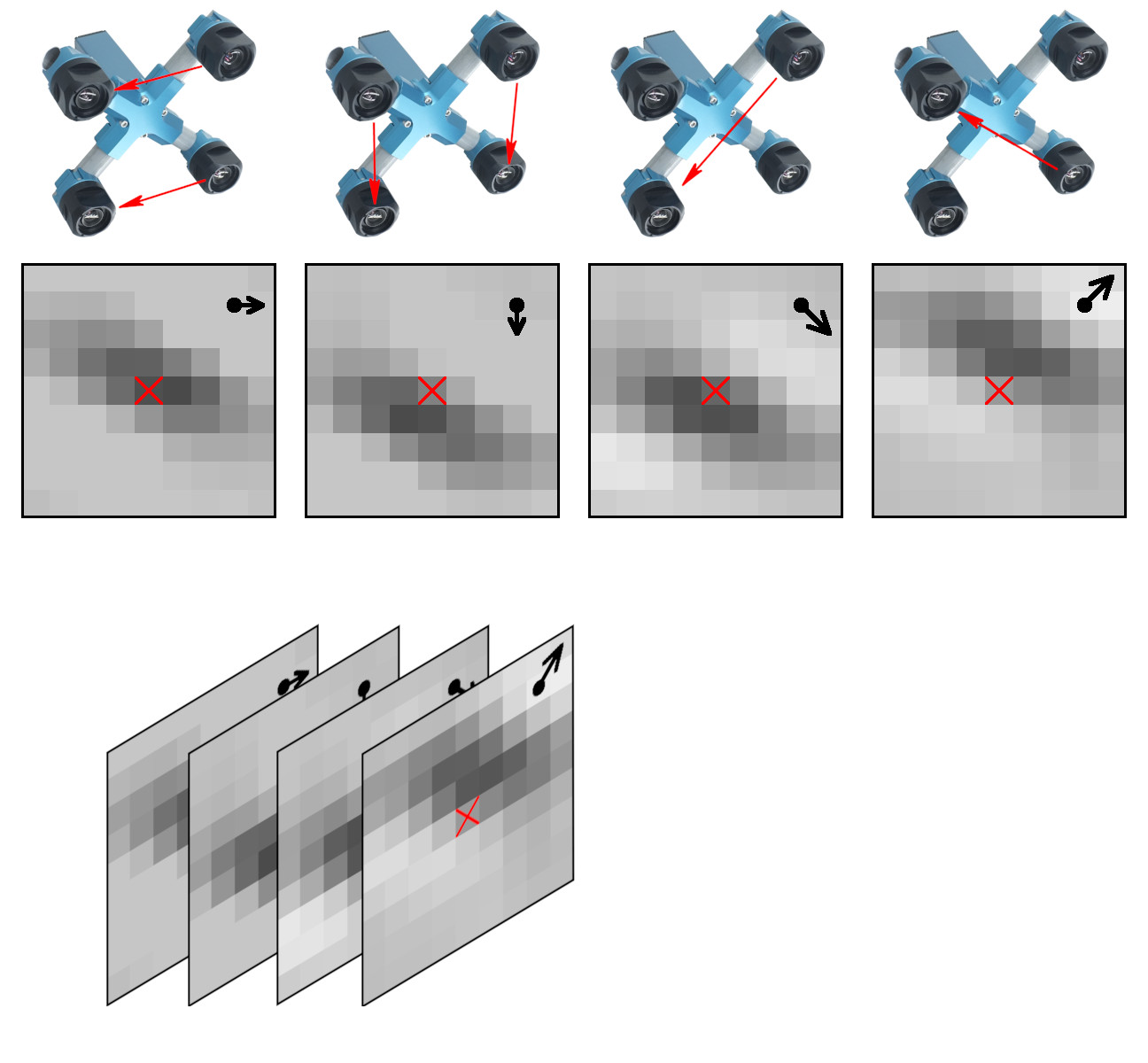
Figure 1. Space-invariant 2D phase correlation data
Data set: source images, 2D correlation tiles, and X3D scene models
The data set contains 2D phase correlation output calculated from the 2592×1936 Bayer mosaic source images captured by the quad stereo camera, and Disparity Space Image (DSI) calculated from a pair of such cameras. Longer baseline provides higher range resolution and this DSI is serving as the ground truth for a single quad camera. The source images as well as all the used software is also provided under the GNU/GPLv3 license. DSI is organized as a 324×242 array – each sample is calculated from the corresponding 16×16 tile. Tiles are overlapping (as shown in Figure 3) with stride 8.
These data sets are provided together with the fully reconstructed X3D scene models, viewable in the browser (Wavefront OBJ files are also generated). The scene models are different from the raw DSI as the next software stages generate meshes, and that frequently leads to over-simplification of the original DSI (so most fronto parallel objects in the scene provide better range accuracy when probed near the bottom). Each scene is accompanied with the multi-layer TIFF file (*-DSI_COMBO.tiff) that allows to see the difference between the measured DSI and the one used in the rendered X3D model. File format and Python import software is documented in Oleg’s post “Reading quad stereo TIFF image stacks in Python and formatting data for TensorFlow”, the data files are directly viewable with ImageJ.
(more…)
Next Page »
 It has been a while since we wrote on the Elphel Development Blog. However, it doesn’t mean we haven’t been developing new technologies and applications. In fact, there is so much new that I would want to write a post for each new project once it is possible, i.e., after Ukraine wins the war.