Long range multi-view stereo camera with 4 sensors
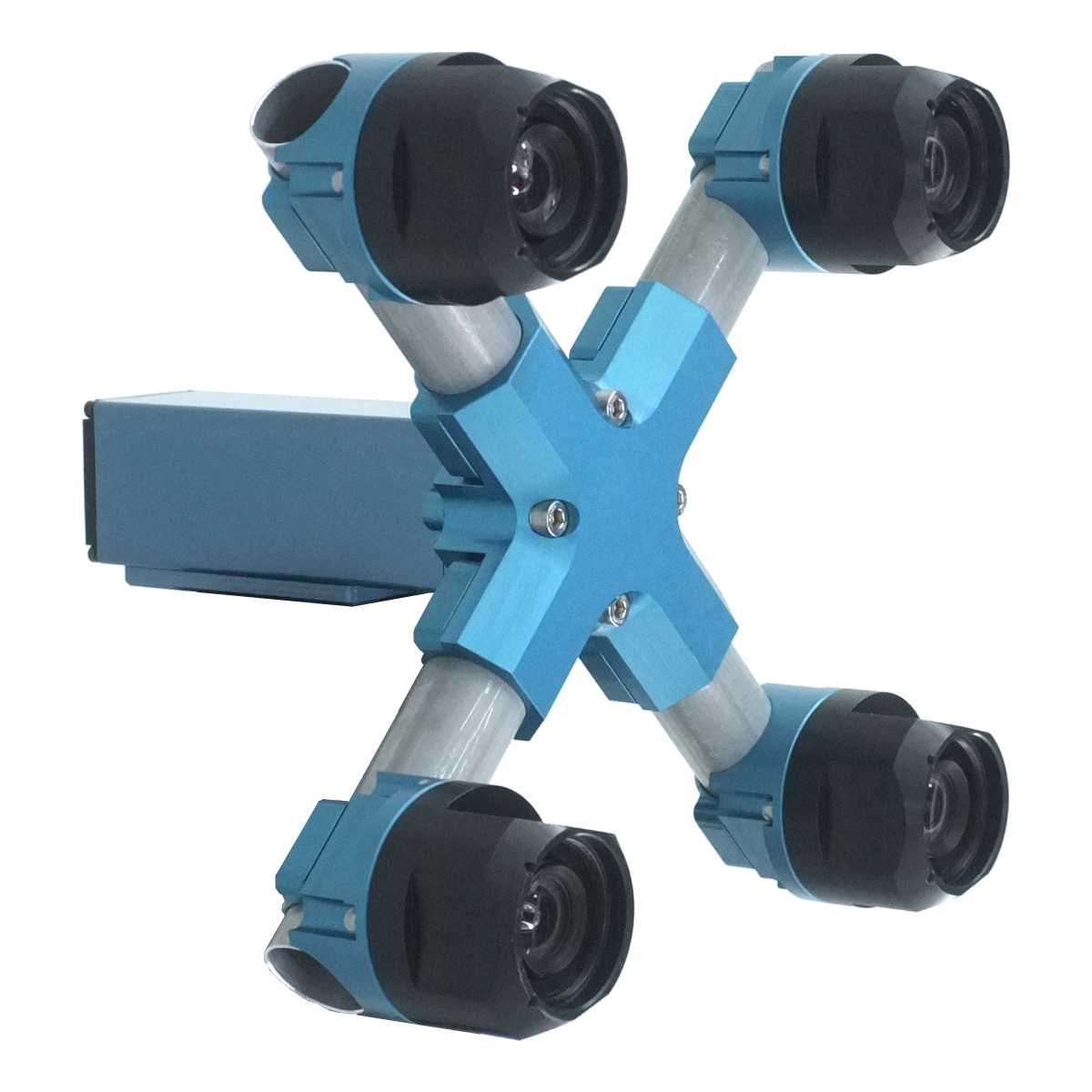
Figure 1. Four sensor stereo camera
Contents
- 1 Background
- 2 Technology snippets
- 2.1 Narrow baseline and subpixel resolution
- 2.2 Subpixel accuracy and the lens distortions
- 2.3 Fixed vs. variable window image matching and FPGA
- 2.4 Two dimensional array vs. binocular and inline camera rigs
- 2.5 Image rectification and resampling
- 2.6 Enhancing images by correcting optical aberrations with space-variant deconvolution
- 2.7 Two dimensional vs. single dimensional matching along the epipolar lines
- 3 Implementation
- 4 Scene viewer
- 5 Results
Scroll down or just hyper-jump to Scene viewer for the links to see example images and reconstructed scenes.
Background
Most modern advances in the area of the visual 3d reconstruction are related to structure from motion (SfM) where high quality models are generated from the image sequences, including those from the uncalibrated cameras (such as cellphone ones). Another fast growing applications depend on the active ranging with either LIDAR scanning technology or time of flight (ToF) sensors.
Each of these methods has its limitations and while widespread smart phone cameras attracted most of the interest in the algorithms and software development, there are some applications where the narrow baseline (distance between the sensors is much smaller, than the distance to the objects) technology has advantages.
Such applications include autonomous vehicle navigation where other objects in the scene are moving and 3-d data is needed immediately (not when the complete image sequence is captured), and the elements to be ranged are ahead of the vehicle so previous images would not help much. ToF sensors are still very limited in range (few meters) and the scanning LIDAR systems are either slow to update or have very limited field of view. Passive (visual only) ranging may be desired for military applications where the system should stay invisible by not shining lasers around.
Technology snippets
Narrow baseline and subpixel resolution
The main challenge for the narrow baseline systems is that the distance resolution is much worse than the lateral one. The minimal resolved 3d element, voxel is very far from resembling a cube (as 2d pixels are usually squares) – with the dimensions we use: pixel size – 0.0022 mm, lens focal length f = 4.5 mm and the baseline of 150 mm such voxel at 100 m distance is 50 mm high by 50 mm wide and 32 meters deep. The good thing is that while the lateral resolution generally is just one pixel (can be better only with additional knowledge about the object), the depth resolution can be improved with reasonable assumptions by an order of magnitude by using subpixel resolution. It is possible when there are multiple shifted images of the same object (that for such high range to baseline ratio can safely be assumed fronto-parallel) and every object is presented in each image by multiple pixels. With 0.1 pixel resolution in disparity (or shift between the two images) the depth dimension of the voxel at 100 m distance is 3.2 meters. And as we need multiple pixel objects for the subpixel disparity resolution, the voxel lateral dimensions increase (there is a way to restore the lateral resolution to a single pixel in most cases). With fixed-width window for the image matching we use 8×8 pixel grid (16×16 pixel overlapping tiles) similar to what is used by some image/video compression algorithms (such as JPEG) the voxel dimensions at 100 meter range become 0.4 m x 0.4 m x 3.2 m. Still not a cube, but the difference is significantly less dramatic.
Subpixel accuracy and the lens distortions
Matching images with subpixel accuracy requires that lens optical distortion of each lens is known and compensated with the same or better precision. Most popular way to present lens distortions is to use radial distortion model where relation of distorted and ideal pin-hole camera image is expressed as polynomial of point radius, so in polar coordinates the angle stays the same while the radius changes. Fisheye lenses are better described with “f-theta” model, where linear radial distance in the focal plane corresponds to the angle between the lens axis and ray to the object.
Such radial models provide accurate results only with ideal lens elements and when such elements are assembled so that the axis of each individual lens element precisely matches axes of the other elements – both in position and orientation. In the real lenses each optical element has minor misalignment, and that limits the radial model. For the lenses we had dealt with and with 5MPix sensors it was possible to get down to 0.2 – 0.3 pixels, so we supplemented the radial distortion described by the analytical formula with the table-based residual image correction. Such correction reduced the minimal resolved disparity to 0.05 – 0.08 pixels.
Fixed vs. variable window image matching and FPGA
Modern multi-view stereo systems that work with wide baselines use elaborate algorithms with variable size windows when matching image pairs, down to single pixels. They aggregate data from the neighbor pixels at later processing stages, that allows them to handle occlusions and perspective distortions that make paired images different. With the narrow baseline system, ranging objects at distances that are hundreds to thousands times larger than the baseline, the difference in perspective distortions of the images is almost always very small. And as the only way to get subpixel resolution requires matching of many pixels at once anyway, use of the fixed size image tiles instead of the individual pixels does not reduce flexibility of the algorithm much.
Processing of the fixed-size image tiles promises significant advantage – hardware-accelerated pixel-level tile processing combined with the higher level software that operates with the per-tile data rather than with per-pixel one. Tile processing can be implemented within the FPGA-friendly stream processing paradigm leaving decision making to the software. Matching image tiles may be implemented using methods similar to those used for image and especially video compression where motion vector estimation is similar to calculation of the disparity between the stereo images and similar algorithms may be used, such as phase-only correlation (PoC).
Two dimensional array vs. binocular and inline camera rigs
Usually stereo cameras or fixed baseline multi-view stereo are binocular systems, with just two sensors. Less common systems have more than two lenses positioned along the same line. Such configurations improve the useful camera range (ability to measure near and far objects) and reduce ambiguity when dealing with periodic object structures. Even less common are the rigs where the individual cameras form a 2d structure.
In this project we used a camera with 4 sensors located in the corners of a square, so they are not co-linear. Correlation-based matching of the images depends on the detailed texture in the matched areas of the images – perfectly uniform objects produce no data for depth estimation. Additionally some common types of image details may be unsuitable for certain orientations of the camera baselines. Vertical concrete pole can be easily correlated by the two horizontally positioned cameras, but if the baseline is turned vertical, the same binocular camera rig would fail to produce disparity value. Similar is true when trying to capture horizontal features with the horizontal binocular system – such predominantly horizontal features are common when viewing near flat horizontal surfaces at high angles of incidents (almost parallel to the view direction).
With four cameras we process four image pairs – 2 horizontal (top and bottom) and 2 vertical (right and left), and depending on the application requirements for particular image region it is possible to combine correlation results of all 4 pairs, or just horizontal and vertical separately. When all 4 baselines have equal length it is easier to combine image data before calculating the precise location of the correlation maximums – 2 pairs can be combined directly, and the 2 others after rotating tiles by 90 degrees (swapping X and Y directions, transposing the tiles 2d arrays).
Image rectification and resampling
Many implementations of the multi-view stereo processing start with the image rectification that involves correction for the perspective and lens distortions, projection of the individual images to the common plane. Such projection simplifies image tiles matching by correlation, but as it involves resampling of the images, it either reduces resolution or requires upsampling and so increases required memory size and processing complexity.
This implementation does not require full de-warping of the images and related resampling with fractional pixel shifts. Instead we split geometric distortion of each lens into two parts:
- common (average) distortion of all four lenses approximated by analytical radial distortion model, and
- small residual deviation of each lens image transformation from the common distortion model
Common radial distortion parameters are used to calculate matching tile location in each image, and while integer rounded pixel shifts of the tile centers are used directly when selecting input pixel windows, the fractional pixel remainders are preserved and combined with the other image shifts in the FPGA tile processor. Matching of the images is performed in this common distorted space, the tile grid is also mapped to this presentation, not to the fully rectified rectilinear image.
Small individual lens deviations from the common distortion model are smooth 2-d functions over the 2-d image plane, they are interpolated from the calibration data stored for the lower resolution grid.
We use low distortion sorted lenses with matching focal lengths to make sure that the scale mismatch between the image tiles is less than tile size in the target subpixel intervals (0.1 pix). Low distortion requirement extends the distances range to the near objects, because with the higher disparity values matching tiles in the different images land to the differently distorted areas. Focal length matching allows to use modulated complex lapped transform (CLT) that similar to discrete Fourier transform (DFT) is invariant to shifts, but not to scaling (log-polar coordinates are not applicable here, as such transformation would deny shift invariance).
Enhancing images by correcting optical aberrations with space-variant deconvolution
Matching of the images acquired with the almost identical lenses is rather insensitive to the lens aberrations that degrade image quality (mostly reduce sharpness), especially in the peripheral image areas. Aberration correction is still needed to get sharp textures in the result 3d models over full field of view, the resolution of the modern sensors is usually better than what lenses can provide. Correction can be implemented with space-variant (different kernels for different areas of the image) deconvolution, we routinely use it for post-processing of Eyesis4π images. The DCT-based implementation is described in the earlier blog post.
Space-variant deconvolution kernels can absorb (be combined with during calibration processing) the individual lens deviations from the common distortion model, described above. Aberration correction and image rectification to the common image space can be performed simultaneously using the same processing resources.
Two dimensional vs. single dimensional matching along the epipolar lines
Common approach for matching image pairs is to replace the two-dimensional correlation with a single-dimensional task by correlating pixels along the epipolar lines that are just horizontal lines for horizontally built binocular systems with the parallel optical axes. Aggregation of the correlation maximums locations between the neighbor parallel lines of pixels is preformed in the image pixels domain after each line is processed separately.
For tile-based processing it is beneficial to perform a full 2-d correlation as the phase correlation is performed in the frequency domain, and after the pointwise multiplication during aberration correction the image tiles are already available in the 2d frequency domain. Two dimensional correlation implies aggregation of data from multiple scan lines, it can tolerate (and be used to correct) small lens misalignments, with appropriate filtering it can be used to detect (and match) linear features.
Implementation
Prototype camera
Experimental camera looks similar to Elphel regular H-camera – we just incorporated different sensor front ends (3d CAD model) that are used in Eyesis4π and added adjustment screws to align optical axes of the lenses (heading and tilt) and orientations of the image sensors (roll). Sensors are 5 Mpix 1/2″ format On Semiconductor MT9P006, lenses – Evetar N125B04530W.
We selected lenses with the same focal length within 1%, and calibrated the camera using our standard camera rotation machine and the target pattern. As we do not yet have production adjustment equipment and software, the adjustment took several iterations: calibrating the camera and measuring extrinsic parameters of each sensor front end, then rotating each of the adjustment screws according to spreadsheet-calculated values, and then re-running the whole calibration process again. Finally the calibration results: radial distortion parameters, SFE extrinsic parameters, vignetting and deconvolution kernels were converted to the form suitable for run-time application (now – during post-processing of the captured images).
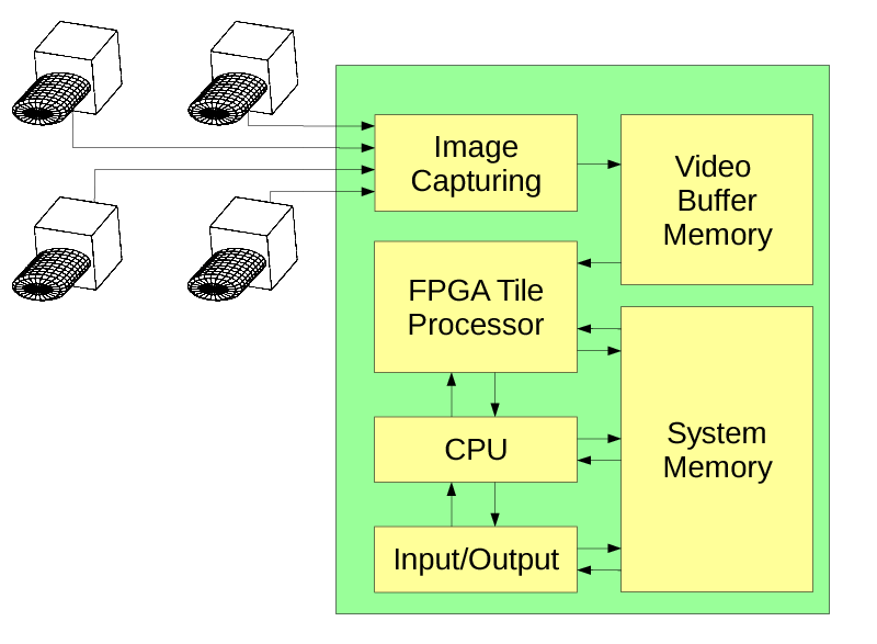
Figure 2. Camera block diagram
This prototype still uses 3d-printed parts and such mounts proved to be not stable enough, so we had to add field calibration and write code for bundle adjustment of the individual imagers orientations from the 2-d correlation data for each of the 4 individual pairs.
Camera performance depends on the actual mechanical stability, software-compensation can only partially mitigate this misalignment problem and the precision of the distance measurements was reduced when cameras went off by more than 20 pixels after being carried in a backpack. Nevertheless the scene reconstruction remained possible.
Software
Multi-view stereo rigs are capable of capturing dynamic scenes so our goal is to make a real-time system with most of the heavy-weight processing be done in the FPGA.
One of the major challenges here is how to combine parallel and stream processing capabilities of the FPGA with the flexibility of the software needed for implementation of the advanced 3d reconstruction algorithms. This approach is to use the FPGA-based tile processor to perform uniform operations on the lists of “tiles” – fixed square overlapping windows in the images. FPGA processes tile data at the pixel level, while software operates the whole tiles.
Figure 2 shows the overall block diagram of the camera, Figure 3 illustrates details of the tile processor.
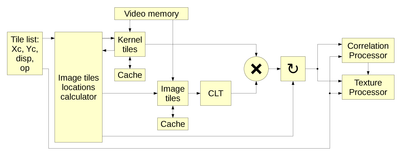
Figure 3. FPGA tile processor
Initial implementation does not contain actual FPGA processing, so far we only tested in FPGA some of the core functions – two dimensional 8×8 DCT-IV needed for both 16×16 CLT and ICLT. Current code consists of the two separate parts – one part (tile processor) simulates what will be moved to the FPGA (it handles image tiles at the pixel level), and the other one is what will remain software – it operates on the tile level and does not deal with the individual pixels. These two parts interact using shared system memory, tile processor has exclusive access to the dedicated image buffer and calibration data.
Each tile is 16×16 pixels square with 8 pixel overlap, software prepares tile list including:
- tile center X,Y (for the virtual “center” image),
- center disparity, so the each of the 4 image tiles will be shifted accordingly, and
- the code of operation(s) to be performed on that tile.

Figure 4. Correlation processor
Tile processor performs all or some (depending on the tile operation codes) of the following operations:
- Reads the tile tasks from the shared system memory.
- Calculates locations and loads image and calibration data from the external image buffer memory (using on-chip memory to cache data as the overlapping nature of the tiles makes each pixel to participate on average in 4 neighbor tiles).
- Converts tiles to frequency domain using CLT based on 2d DCT-IV and DST-IV.
- Performs aberration correction in the frequency domain by pointwise multiplication by the calibration kernels.
- Calculates correlation-related data (Figure 4) for the tile pairs, resulting in tile disparity and disparity confidence values for all pairs combined, and/or more specific correlation types by pointwise multiplication, inverse CLT to the pixel domain, filtering and local maximums extraction by quadratic interpolation or windowed center of mass calculation.
- Calculates combined texture for the tile (Figure 5), using alpha channel to mask out pixels that do not match – this is the way how to effectively restore single-pixel lateral resolution after aggregating individual pixels to tiles. Textures can be combined after only programmed shifts according to specified disparity, or use additional shift calculated in the correlation module.
- Calculates other integral values for the tiles (Figure 5), such as per-channel number of mismatched pixels – such data can be used for quick second-level (using tiles instead of pixels) correlation runs to determine which 3d volumes potentially have objects and so need regular (pixel-level) matching.
- Finally tile processor saves results: correlation values and/or texture tile to the shared system memory, so software can access this data.

Figure 5. Texture processor
Single tile processor operation deals with the scene objects that would be projected to this tile’s 16×16 pixels square on the sensor of the virtual camera located in the center between the four actual physical cameras. The single pass over the tile data is limited not just laterally, but in depth also because for the tiles to correlate they have to have significant overlap. 50% overlap corresponds to the correlation offset range of ±8 pixels, better correlation contrast needs 75% overlap or ±4 pixels. The tile processor “probes” not all the voxels that project to the same 16×16 window of the virtual image, but only those that belong to the certain distance range – the distances that correspond to the disparities ±4 pixels from the value provided for the tile.
That means that a single processing pass over a tile captures data in a disparity space volume, or a macro-voxel of 8 pixels wide by 8 pixels high by 8 pixels deep (considering the central part of the overlapping volumes). And capturing the whole scene may require multiple passes for the same tile with different disparity. There are ways how to avoid full range disparity sweep (with 8 pixel increments) for all tiles – following surfaces and detecting occlusions and discontinuities, second-level correlation of tiles instead of the individual pixels.
Another reason for the multi-pass processing of the same tile is to refine the disparity measured by correlation. When dealing with subpixel coordinates of the correlation maximums – either located by quadratic approximation or by some form of center of mass evaluation, the calculated values may have bias and disparity histograms reveal modulation with the pixel period. Second “refine” pass, where individual tiles are shifted by the disparity measured in the previous pass reduces the residual offset of the correlation maximum to a fraction of a pixel and mitigates this type of bias. Tile shift here means a combination of the integer pixel shift of the source images and the fractional (in the ±0.5 pixel range) shift that is performed in the frequency domain by multiplication by the cosine/sine phase rotator.
Total processing time and/or required FPGA resources linearly depend on the number of required tile processor operations and the software may use several methods to reduce this number. In addition to the two approaches mentioned above (following surfaces and second-level correlation) it may be possible to reduce the field of view to a smaller area of interest, predict current frame scene from the previous frames (as in 2d video compression) – tile processor paradigm preserves flexibility of the various algorithms that may be used in the scene 3d reconstruction software stack.
Scene viewer
The viewer for the reconstructed scenes is here: https://community.elphel.com/3d+map (viewer source code).

Figure 6. 3d+map index page
Index page shows a map (you may select from several providers) with the markers for the locations of the captured scenes. On the left there is a vertical ribbon of the thumbnails – you may scroll it with a mouse wheel or by dragging.
Thumbnails are shown only for the markers that fit on screen, so zooming in on the map may reduce number of the visible thumbnails. When you select some thumbnail, the corresponding marker opens on the map, and one or several scenes are shown – one line per each scene (identified by the Unix timestamp code with fractional seconds) captured at the same locations.
The scene that matches the selected thumbnail is highlighted (as 4-th line in the Figure 6). Some scenes have different versions of reconstruction from the same source images – they are listed in the same line (like first line in the Figure 6). Links lead to the viewers of the selected scene/version.
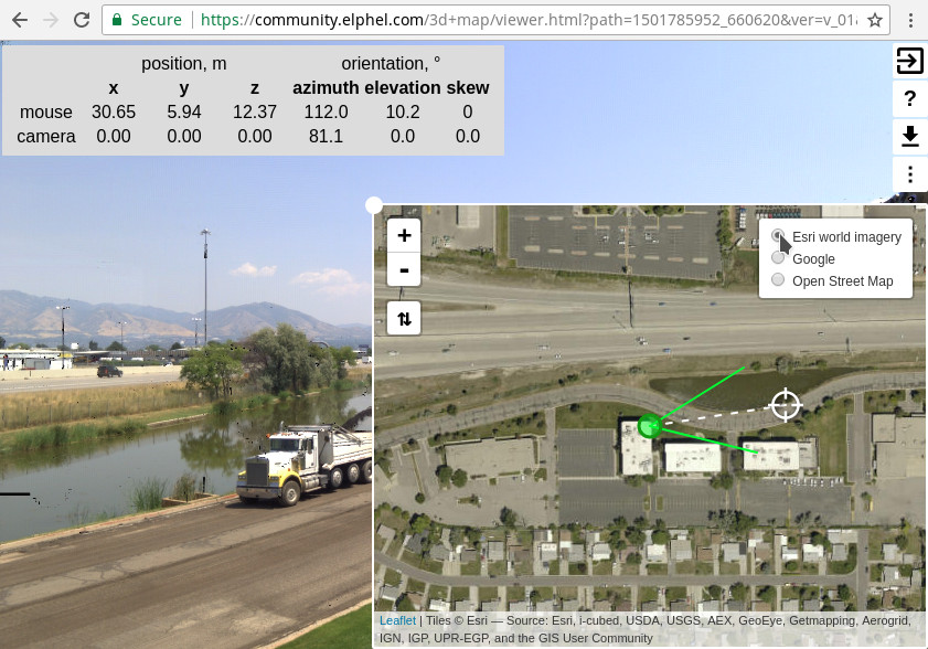
Figure 7. Selection of the map / satellite imagery provider
We do not have ground truth models for the captured scenes build with the active scanners. Instead as the most interesting is ranging of the distant objects (hundreds of meters) it is possible to use publicly available satellite imagery and match it to the captured models. We had ideal view from Elphel office window – each crack on the pavement was visible in the satellite images so we could match them with the 3d model of the scene. Unfortunately they ruined it recently by replacing asphalt :-).
The scene viewer combines x3dom representation of the 3d scene and the re-sizable overlapping map view. You may switch the map imagery provider by clicking on the map icon as shown in the Figure 7.
The scene and map views are synchronized to each other, there are several ways of navigation in either 3d or map area:
- drag the 3d view to rotate virtual camera without moving;
- move cross-hair ⌖ icon in the map view to rotate camera around vertical axis;
- toggle ⇅ button and adjust camera view elevation;
- use scroll wheel over the 3d area to change camera zoom (field of view is indicated on the map);
- drag with middle button pressed in the 3d view to move camera perpendicular to the view direction;
- drag the the camera icon (green circle) on the map to move camera horizontally;
- toggle ⇅ button and move the camera vertically;
- press a hotkey t over the 3d area to reset to the initial view: set azimuth and elevation same as captured;
- press a hotkey r over the 3d area to set view azimuth as captured, elevation equal to zero (horizontal view).
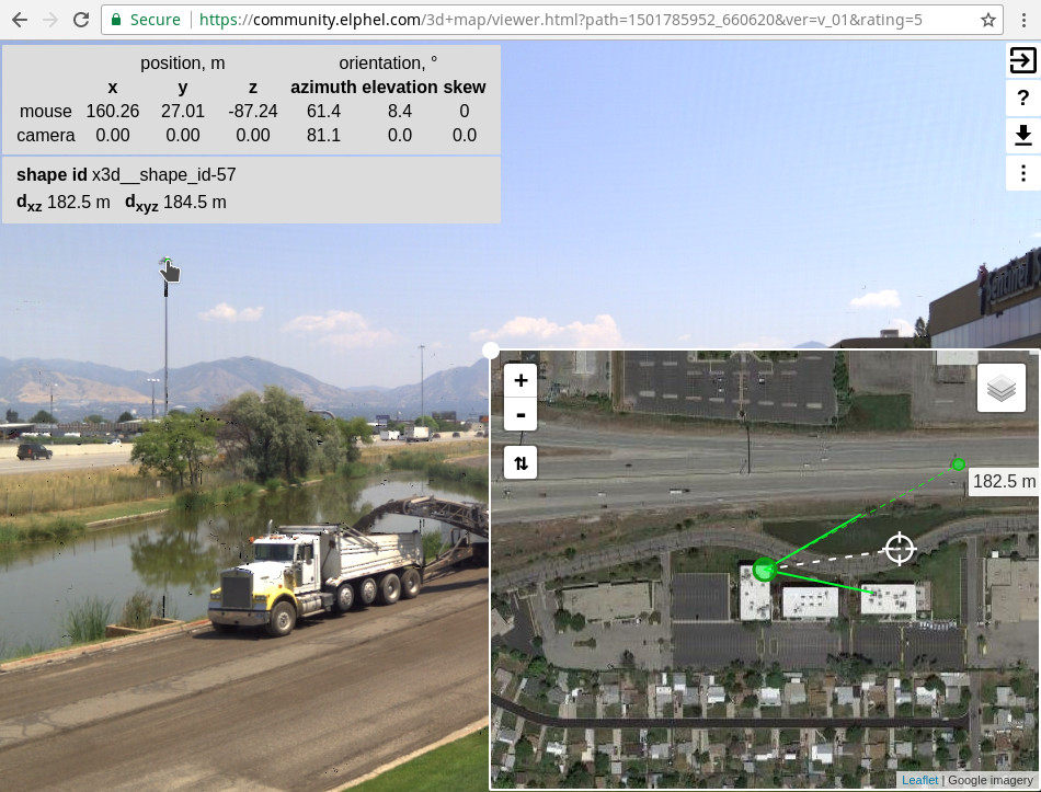
Figure 8. 3D model to map comparison
Comparison of the 3d scene model and the map uses ball markers. By default these markers are one meter in diameter, the size can be changed on the settings (⋮) page.
Moving pointer over the 3d area with Ctrl key pressed causes the ball to follow the cursor at a distance where the view line intersects the nearest detected surface in the scene. It simultaneously moves the corresponding marker over the map view and indicates the measured distance.
Ctrl-click places the ball marker on the 3d scene and on the map. It is then possible to drag the marker over the map and read the ground truth distance. Dragging the marker over the 3d scene updates location on the map, but not the other way around, in edit mode mismatch data is used to adjust the captured scene location and orientation.
Program settings used during reconstruction limit the scene far distance to z = 1000 meters, all more distant objects are considered to be located at infinity. X3d allows to use images at infinity using backdrop element, but it is not flexible enough and is not supported by some other programs. In most models we place infinity textures to a large billboard at z = 10,000 meters, and it is where the ball marker will appear if placed on the sky or other far objects.
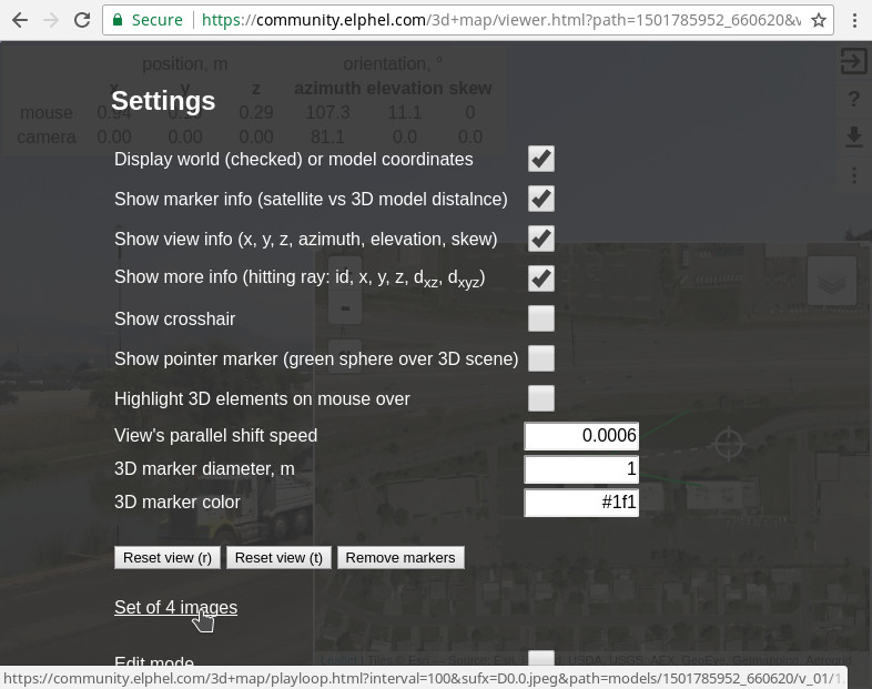
Figure 9. Settings and link to four images
The settings page (⋮) shown in the Figure 9 has a link to the four-image viewer (Figure 10). These four images correspond to the captured views and are almost “raw images” used for scene reconstruction. These images were subject to the optical aberration correction and are partially rectified – they are rendered as if they were captured by the same camera that has only strictly polynomial radial distortion.
Such images are not actually used in the reconstruction process, they are rendered only for the debug and demonstration purposes. The equivalent data exists in the tile processor only in the frequency domain form as an intermediate result, and was subject to just linear processing (to avoid possible unintended biases) so the images have some residual locally-checkerboard pattern that is due to the Bayer mosaic filter (discussed in the earlier blog). Textures that are generated from the combination of all four images have the contrast of such pattern significantly lower. It is possible to add some non-linear filtering at the very last stage of the texture generation.
Each scene model has a download link for the archive that contains the model itself as *.x3d file and Wavefront *.obj and *.mtl as well as the corresponding RGBA texture files as PNG images. Initially I missed the fact that x3d and obj formats have opposite direction of surface normals for the same triangular faces, so almost half of the Wavefront files still have incorrect (opposite direction) surface normals.
Results
Our initial plan was to test algorithms for the tile processor before implementing them in FPGA. The tile processor provides data for the disparity space image (DSI) – confidence value of having certain disparity for specified 2d position in the image, it also generates texture tiles.
When the tile processor code was written and tested, we still needed some software to visualize the results. DSI itself seemed promising (much better coverage than what I had with earlier experiments with binocular images), but when I tried to convert these textured tiles into viewable x3d model directly, it was a big disappointment. Result did not look like a 3d scene – there were many narrow triangles that made sense only when viewed almost directly from the camera actual location, a small lateral viewpoint movement – and the image was falling apart into something unrecognizable.

Figure 10. Four channel images (click for actual viewer with zoom/pan capability)
I was not able to find ready to use code and the plan to write a quick demo for the tile processor and generated DSI seemed less and less realistic. Eventually it took at least three times longer to get somewhat usable output than to develop DCT-based tile processor code itself.
Current software is still incomplete, lacks many needed features (it even does not cut off background so wires over the sky steal a lot of surrounding space), it runs slow (several minutes per single scene), but it does provide a starting point to evaluate performance of the long range 4-camera multi-view stereo system. Much of the intended functionality does not work without more parameter tuning, but we decided to postpone improvements to the next stage (when we will have cameras that are more stable mechanically) and instead try to capture more of very different scenes, process them in batch mode (keeping the same parameter values for all new scenes) and see what will be the output.
As soon as the program was able to produce somewhat coherent 3d model from the very first image set captured through Elphel office window, Oleg Dzhimiev started development of the web application that allows to match the models with the map data. After adding more image sets I noticed that the camera calibration did not hold. Each individual sub-camera performed nicely (they use thermally compensated mechanical design), but their extrinsic parameters did change and we had to add code for field calibration that uses image themselves. The best accuracy in disparity measurement over the field of view still requires camera poses to match ones used at full calibration, so later scenes with more developed misalignment (>20 pixels) are less precise than earlier (captured in Salt Lake City).
We do not have an established method to measure ranging precision for different distances to object – the disparity values are calculated together with the confidence and in lower confidence areas the accuracy is lower, including places where no ranging is possible due to the complete absence of the visible details in the images. Instead it is possible to compare distances in various scene models to those on the map and see where such camera is useful. With 0.1 pixel disparity resolution and 150 mm baseline we should be able to measure 300 m distances with 10% accuracy, and for many captured scene objects it already is not much worse. We now placed orders to machine the new camera parts that are needed to build a more mechanically stable rig. And parallel to upgrading the hardware, we’ll start migrating the tile processor code from Java to Verilog.
And what’s next? Elphel goal is to provide our users with the high performance hackable products and freedom to modify them in the ways and for the purposes we could not imagine ourselves. But it is fun to fantasize about at least some possible applications:
- Obviously, self-driving cars – increased number of cameras located in a 2d pattern (square) results in significantly more robust matching even with low-contrast textures. It does not depend on sequential scanning and provides simultaneous data over wide field of view. Calculated confidence of distance measurements tells when alternative (active) ranging methods are needed – that would help to avoid infamous accident with a self-driving car that went under a truck.
- Visual odometry for the drones would also benefit from the higher robustness of image matching.
- Rovers on Mars or other planets using low-power passive (visual based) scene reconstruction.
- Maybe self-flying passenger multicopters in the heavy 3d traffic? Sure they will all be equipped with some transponders, but what about aerial roadkills? Like a flock of geese that forced water landing.
- High speed boating or sailing over uneven seas with active hydrofoils that can look ahead and adjust to the future waves.
- Landing on the asteroids for physical (not just Bitcoin) mining? With 150 mm baseline such camera can comfortably operate within several hundred meters from the object, with 1.5 m that will scale to kilometers.
- Cinematography: post-production depth of field control that would easily beat even the widest format optics, HDR with a pair of 4-sensor cameras, some new VFX?
- Multi-spectral imaging where more spatially separate cameras with different bandpass filters can be combined to the same texture in the 3d scene.
- Capturing underwater scenes and measuring how far the sea creatures are above the bottom.
- …
Update: We’ve got machined parts to assemble the cameras shown only as a CAD rendering on Figure 1.
> “Vertical concrete pole can be easily correlated by the two horizontally positioned cameras, but if the baseline is turned vertical, the same binocular camera rig would fail to produce disparity value.”
…
> “With four cameras we process four image pairs – 2 horizontal (top and bottom) and 2 vertical (right and left), and depending on the application requirements for particular image region it is possible to combine correlation results of all 4 pairs, or just horizontal and vertical separately.”.
Similarly, if the baseline is turned diagonally, the same quadocular camera rig would fail to produce disparity value if you only use left/right and up/down algorithms.
If you also use the 2 sets of diagonally placed cameras (in your 4 Camera setup) you get twice as much Data without any additional Hardware – with only two Cameras nothing can be done but with you Triclops and Quadocular Cameras you can pair-up additional combinations to wrestle a lot more Data out of the Hardware and obtain a huge improvement over what is possible with binocular (and ‘double-binocular’) vision.
Rob, it is possible to make a tilted line detector using the same 2-d correlation results, but vertical and horizontal features are more common in the real scenes than arbitrary angles. And when combining correlation results from 2 or 4 pairs I use offset multiplication to balance between averaging (lower noise but more false positives) and pure multiplication (same local disparity maximum should appear an all 4 or 2 pairs) that is more dependent on noise, but produces less false-positives.
Here is how I use 2 horizontal pairs combined (multiplied with specified offset). I have a vertical pole at 200 meters that corresponds to 1.5 pixel disparity and far background with disparity 0. Correlation for vertical pairs will not produce anything from the pole, just a maximum at (0,0) from the background. Two horizontal pairs will also produce same spot at (0,0) and a vertical line at x=1.5. The correlation value for that line can be much lower than the maximum at (0,0) and I use a notch filter – zero out everything for say -1 ≤ y ≤ 1 and sum each column – the result will have maximum at x=1.5 (using quadratic interpolation or center of mass with window to subdivide integer grid) . Considering all 4-pair correlation (producing maximum at 0) and horizontal pairs that result in x=1.5 it is possible to separate foreground from the textured background.
I did not play much with arbitrary direction line detection – it can be implemented by tilted notch filter and summation of the 2-d correlation data.
Adding 2 diagonal pairs to the two vert/hor ones will not give any new data as they are dependent. Using them instead (2 pairs instead of 4) would prevent using non-linear combining of the 2 correlations (disparity maximum should appear on each of the pairs to count).
Really impressive and interesting work. One question – if a user was primarily interested in the depth data and not the original colour image, do you think using monochrome sensors would improve the results ?
The argument for would be that raw pixels are going into the DCT, not de-Bayered RGB, and this gives better precision ( I assume this is the current implementation but could be wrong ). The argument against would be that the 3 channels provide sufficiently more interesting information that it makes the correlation work better. Anyway just a thought. Thanks
Jim, I did not try a monochrome sensor, and you are right – while it may be possible to slightly increase subpixel resolution with the monochrome sensor, color data reduces ambiguity of matching.
In the case of the monochrome sensor we would have to use a bandpass filter (such as green), otherwise lens chromatic aberration would reduce the overall resolution in the off-center areas of the image. When processing each color channel individually, we correct chromatic aberration.
And we are trying to get a free ride on the phone cameras boom – use the sensors perfected for such applications. And they are all color, of course.
Is there any benefit at all on co-linear cameras? either horizontal or vertical? what about a mixed system with a Y setup, or maybe a Y inverted, or even a 90 degree rotated Y setup, three cameras within a circle in a 120 degrees separated angle setup. and a fourth central camera so you have a two vertical and two horizontal aligned cameras. but their alignment doesn’t meet in the centre of the setup. With the central camera you could capture the actual colours of the centre and enhance them with the 3d-ness of the 3 other cameras. Would it be any useful beside the squared system like the one you presented?
Biel, I see in-line arrangement to have advantages in 2 areas:
Other (not co-linear) arrangements can better handle occlusions. Horizontal object – a wire, a tree branch will still cover the background object, you can not post-focus on it without “guessing” (modern AI algorithms are really good at it, but still) the missing elements – imagine filming and focusing on a human face behind thin branches. Another advantage for such setup is that it can measure disparity (and so distance) to the objects that do not have (or have poor) vertical features on the texture – there are many such cases in both natural and artificial environments. It is even possible to use the difference between correlation in different directions for filtering and discriminating scene objects.
And yes, there are many configurations of the cameras, and having multiple cameras filming the same object has another advantage when using modern small-pixel sensors – combining data from them improves dynamic range, reduces noise, and makes image quality competitive with the large-pixel cameras. And you may implement simultaneous HDR by combining from spatially offset cameras (using calculated textures, not the raw 2d images).
Square setup simplifies calculations, especially in the FPGA (or eventually VLSI), combining orthogonal, equal baseline correlation involves just matrix transposition (changing the samples order) without any additional DSP operations. And I’m now making good progress in converting Java code (already tested) to Verilog :-).
[…] source Elphel camera unveils its 4-way camera device that is said to have higher depth resolution and less prone to artifacts than stereo […]