Neural network doubled effective baseline of the stereo camera
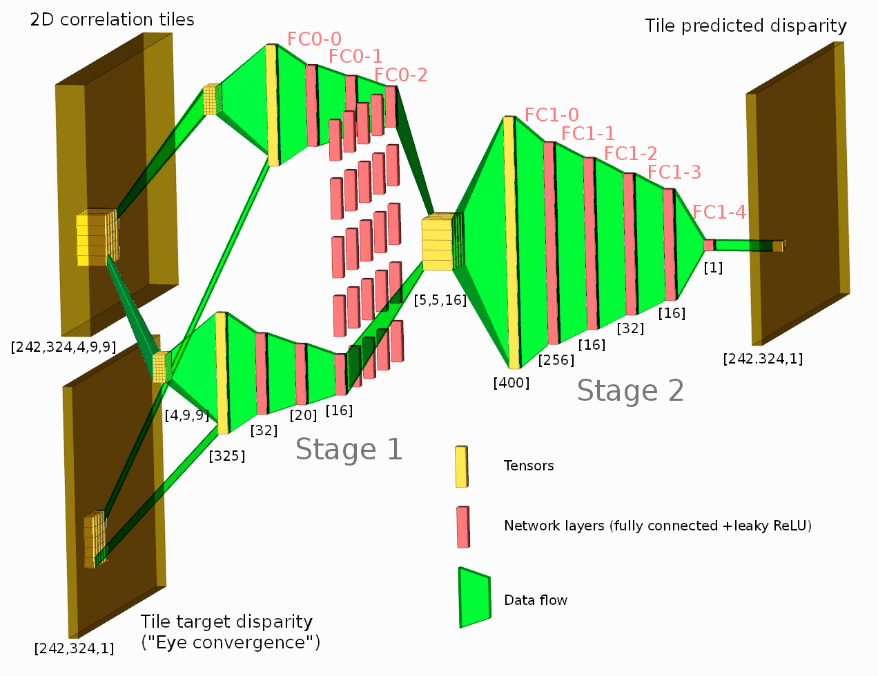
Figure 1. Network diagram. One of the tested configurations is shown.
Neural network connected to the output of the Tile Processor (TP) reduced the disparity error twice from the previously used heuristic algorithms. The TP corrects optical aberrations of the high resolution stereo images, rectifies images, and provides 2D correlation outputs that are space-invariant and so can be efficiently processed with the neural network.
What is unique in this project compared to other ML applications for image-based 3D reconstruction is that we deal with extremely long ranges (and still wide field of view), the disparity error reduction means 0.075 pix standard deviation down from 0.15 pix for 5 MPix images.
See also: arXiv:1811.08032
Contents
Tile Processor and the 2D correlation output
TP receives raw Bayer mosaic data from four (or more) camera sensors and combines several chained operations in the frequency domain, eliminating re-sampling errors. TP operates with the fixed windows of 16×16 Bayer mosaic pixels (stride 8 in each direction). While the camera does not have any moving parts, TP operates similarly to the human vision – it calculates correlations for the requested “target disparity” that is analogous to the eye convergence. The difference is that each image tile may have independently set target disparity.
At this stage of the project we evaluated generation of the depth map using 2D correlation outputs for the tiles and the tile target disparity. Of the six possible correlation pairs of the four camera sensors (top, bottom, left, right and two diagonals) we used four, combining (by averaging) horizontal and vertical pairs together. Of the full 2D correlation results we preserved the center 9×9 pixels, so each tile provides 4×9×9 tensor as shown in Figure 1. Five megapixel sensors output 2592(H)×1936(V) pixels making it 324(H)×242(V) tiles. Target disparity for each tile is calculated using existing heuristic-based program, and the network is trained to improve that value using the 2D correlation data.
Neural network and the data sets
Suggested network architecture consists of the two stages – first stage processes each tile output without any interaction with the neighbors, the second will be convolutional enhancing disparity prediction for each tile by using information from the neighbors. We now use a Siamese type network with samples combining correlation outputs (and corresponding target disparities) from 5×5 tile regions, with network trained to predict disparity of the center tile only. While it is less efficient when processing continuous depth maps, it gives us higher training flexibility by allowing to adjust frequency of the “smooth” samples and the samples with discontinuities of different types.
We had 266 processed scenes to use for training and testing. Each scene provides up 324×242=78408 tiles, of them about half are usable (not the featureless sky and not the near objects that we did not used in this project). When capturing images camera was running at 5 frames per second, so we put aside first image from each second for testing (20%) and used the rest for training. Trying to equalize batches we calculated 2D histogram (disparity-confidence) over all images, divided disparity-confidence area into equal percentile regions and then created batches from the data files selecting random tiles – one from each of those regions.
For the ground truth we used disparity/confidence pairs captured by a dual camera rig that has a baseline almost 5 times longer than that of a single camera. Initial cost function was just a weighted (by ground truth confidence) squared disparity difference, later we clipped it by a certain value to reduce influence of a rather common case when the dual camera rig measurement (ground truth) and that of a single camera (used as target disparity) matched different (foreground or background) objects for the same tile resulting in multi-pixel disparity differences.
The training results were evaluated in 2 ways. First we compared costs (total one minimized and partials) for the training data, test data independently generated but from the same source files already used for training, and from the fresh images that were laid aside for testing. Difference between the tests was used as an indication of overfitting. In addition we compared the heuristic output for the whole test images (same data was also used as a target disparity input for the network) and the network output, calculating accuracy gain for different criteria: tiles with certain disparity range and correlation strength (confidence). And it is this gain for far tiles (less than 5 pix disparity or farther than 100 meters) that let us claim that the network doubled disparity resolution that is equivalent of using twice longer baseline of the stereo camera.
Noticing that overfitting starts to develop (by comparing costs corresponding to the test data) we performed the following actions:
- Applied right/left mirroring of the source data. There may be insufficient up/down and transposition symmetry so we did not rely on replicating source data that way
- First layer of the stage 1 subnets receives image-like 2D correlation data that has certain properties, so for regularization we added costs for the Laplacians of the first layer relative weights with the zero boundary conditions
- Processing in the stage 2 should provide reasonable results even when only the data from the same (center) tile is available. Adding 8 (for 3×3 kernel) neighbors and then 16 (to the total of 5×5) should improve result, so we added 2 more instances (sharing all weights) of the stage 2 – one with all zeros but the center (of 25 stage 1 subnets) input, and the other with the center 3×3 non-zero inputs. And then calculated cost for the error of each of these outputs and mixed them in the final cost used for optimization.
These methods combined allowed to postpone the beginning of overfitting and improved convergence – the results did not go worse (at least significantly) when the training ran for too long.

Results
Figures 2 and 3 illustrate results of the depth map processing with the neural network. Each has 6 sub plots following the common pattern:
- Top right “Ground truth confidence” contains the full scene correlation strength and the red frame that identifies what part of the scene is analyzed in the other subplots
- Top left “Ground truth disparity map” shows tile disparity values as measured by a wide baseline dual camera rig. The disparity units as shown on the vertical bar to the right are pixels of the main camera (not the long baseline rig), same units are used on all the remaining subplots
- Middle left “Heuristic disparity map” shows result of the existing processing of the 2D tile correlation output using heuristic algorithms. These values are used as “target disparity” to calculate 2D correlation for each tile and the correlation results (as 4×9×9 tensors) are fed to the network.
- Bottom left “Network disparity output” shows the network output for the tiles that do have ground truth data, tiles output that can not be verified is blanked (shown in white)
- Middle right shows mismatch between the heuristic disparity map (middle left) and the ground truth disparity (top left)
- Bottom right shows similar errors of the network disparity prediction
Image captions provide the links to the x3d models of the same scene (models are built with the existing software that uses what is considered here as “ground truth” and do not rely on the network processing). Another link (Images↗) in the captions leads to the camera image viewer for the scene. That viewer shows all 8 camera images, the first 4 correspond to the processed data, the last 4 are captured by a second camera used for the ground truth measurements. These images are not raw (raw Bayer mosaic images are also provided as explained in the wiki page), they are calculated for the target disparity set to 0 for all tiles. Images are the result of the space-variant deconvolution for aberration correction, they are being subject to the linear operations only, so at certain zoom levels they have visible modulation caused by the Bayer mosaic, and color de-mosaic artifacts in the periodic grid areas as there are no (nonlinear) demosaic operations in the processing pipeline.

Evaluating disparity maps of the flat horizontal surface
The scene fragment in Figure 2 shows rather flat surface from 1000 meters (~0.5 pix disparity) to infinity (mountain ridge is over 20,000 meters – beyond the resolution of the camera). The disparity noise of the middle row (heuristic output) is greatly reduced by the network (bottom row) and it is not just the low-pass filtering – the transition to the near objects (yellow) is not blurred. The network output reveals some low frequency disparity fluctuations that are not present in the ground truth data (top subplot). These fluctuations are caused by the correlations between the Bayer patterns of the individual sensors, each pattern being distorted by the optical aberration correction. These errors may be reduced by feeding all 6 individual correlation pairs to the network – currently two horizontal (top and bottom) and two vertical (left and right) pairs are reduced by averaging. Combining them non-linearly in the network may increase S/N ratio. Additionally this noise may be reduced by adding more sensors without increasing the overall camera dimensions.
Disparity maps in the urban environment
Figure 3 contains the scene fragment captured while driving northbound along the State Street in Salt Lake City. The buildings visible there (pseudo-colors other than white and yellow) are from 680 meters to 2200 meters ahead (2200 m is the Utah State Capitol around tile at [170,113] – it is visible on the ground truth (top left) and network output (bottom left) subplots.
The challenge here was to prevent the network from blurring the depth map between objects at different distances. While smooth disparity gradients are possible (like the street pavement) most detectable disparity variations at long distances are due to the discontinuities caused by the overlapping objects. When disparity difference is small (1 pixel or less) the correlation argmax for the tile containing both foreground and background pixels would be (incorrectly) somewhere between the foreground and the background values. For the purpose of the next stage of the scene 3d reconstruction – fitting planes – it would be better if such edge tile would be assigned to either foreground or background. And this “cutting corners” on the depth map did happen with the initial cost function based on L2 (cost proportional to squared difference to ground truth disparity weighted with the ground truth confidence) alone.
Cost function for preserving edges in the depth map
Tweaking the cost function significantly improved performance – the result is visible by comparing middle right and bottom right subplots along the vertical building edge at horizontal tile 163 and vertical between 100 and 111 of the Figure 3. The difference between the heuristic disparity and the ground truth shows a visible tile column that is more negative than the tiles around it (the disparity of the foreground object was reduced by correlation). That column completely disappears in the bottom right subplot as the edge sharpness is restored by the trained network.
The cost function was modified in the following way:
- First the disparity difference was leaky-clipped to 0.3 pixels. Larger errors are usually caused by matching different objects – ground truth may be measured for the distant background while the target disparity matched closer foreground (or vice versa).
- The second modification specifically added extra cost for “cutting corners” (blurring edges). The average value of the 8 neighbors’ ground truth disparity is calculated for each tile, and outputs falling between the ground truth disparity and the average disparity generate additional cost.
Next steps
Increase of the depth resolution twice was just a low hanging fruit – this project is our first hands-on experience with the neural networks. When visitors of our booth at CVPR-2018 were amazed by just a few percents range error at 2000 meters in the interactive X3D model, we had to explain that the model uses data captured by a pair of such cameras and we plan to use it as a ground truth for the neural network training. And that we hope that eventually a single 258 mm quad camera using the neural network will provide the data as accurate as the existing dual camera rig with 1256 mm baseline. We are not there yet, just half-way, but believe that our original estimate was correct and that goal is reachable.
Add more data
The next immediate step will be adding more training data and possibly reimplementing the TP code to use GPU (this code exist now in Java for CPU and in Verilog for FPGA/VLSI). CPU TP implementation is a bottleneck in the current pipeline, so far we processed only few percents of the captured imagery. Larger dataset will allow to try deeper/wider networks
We will evaluate results of feeding all 6 pairs to the network and experiment with cost functions to reduce noise caused by the correlation of the Bayer patterns of the individual sensors
and maintain space-invariance of the TP output.
Generate output for field calibration
Currently the network outputs only the single scalar per each tile – disparity value. It is important to train the network to generate the confidence value of the disparity it outputs. Additionally the heuristic program we use now can provide misalignment data for each tile (“lazy eye”) – such data is used for field calibration of the camera system by bundle adjustment of the individual sensors attitude. Such output can also be received from the network.
Then we will work on switching other parts of the 3d scene reconstruction to use the neural networks and there are at least two areas that rely not just on straightforward math but use a lot of heuristics.
Target disparity calculation with NN
One such area is selection of the target disparity for each tile. With the small TP window the correlation output provides valid result only within just a few disparity pixels of the center – preprogrammed shift. Full disparity sweep would be expensive so current software uses a combination of methods – scans all tiles at infinity, then uses that data to create low resolution images and correlates them to identify potentially occupied 3D volumes, then grows measured tiles by predicting disparity for the new tiles and measuring correlation. This prediction depends heavily on heuristics and seems to be a good application area to use the network.
Building 3D surfaces
Another area is building 3D surfaces from tile disparities, it is highly heuristic-infested too. Current software uses “supertiles” (overlapping areas of 16×16 with stride 8 tiles) to build multiple “plates” using eigenvalues/eigenvectors of the covariance matrices build of the tile data. Then such plates in the neighboring supertiles are matched to each other and merged if they are likely to belong to the same 3D surface. These plates simultaneously use both the Disparity Space Image (DSI) and the world 3D coordinates. The DSI coordinates are native to the camera and the measurement accuracy can be expressed in the pixels of DSI. The real world coordinates, on the other hand characterize likelihood of such 3d object to exist. The plate merging considers both DSI distance (to be withing measurement accuracy) and world 3D (comparing angles and linear distances between planes to merge). After merging the supertile plates into 3D surfaces, each tile is re-evaluated and assigned to one of them.
Pixel-accurate texture edges
The last step of building realistic 3D scene models was not implemented in the current software – just the provisions for it in the tile processor. It is the restoration of the pixel-accurate edges in the output textures from the tile-accurate depth map and the texture tiles output from the TP.
Hardware improvements
In parallel we plan to improve the hardware and the image capturing process. We will make a light enclosure and a more rigid frame to eliminate the need for additional field calibration, caused by minor variations (mostly thermal) of the camera sensors attitudes. We will try to use fusion of multiple scene models to calculate 3D ground truth data instead of the dual camera rig that we use now. This rig relies on the really far objects (tens of thousands meters) to be able to calibrate itself. We are lucky to have mountain ridges visible around in Salt Lake City, but even they are often too close to be considered infinity.
A fun project
And a fun project – we will try to capture a flock of birds in the air and see how well we can measure and track the 3D coordinates of the multitude of the small flying objects – both without and with the neural network.
Leave a Reply