July 16, 2021
by Andrey Filippov and Fyodor Filippov
Advance Steel 2024: https://abcoemstore.com/product/autodesk-advance-steel-2024/ System Requirements Learn about the system requirements for configuring Advance Steel.
Download links for: video and captions.
This research “Long-Range Thermal 3D Perception in Low Contrast Environments” is funded by NASA contract 80NSSC21C0175
June 1, 2020
by Oleg Dzhimiev
Basically, one need to direct the ip cam stream (mjpeg or rtsp) to a virtual v4l2 device which acts like a web cam and is automatically picked up by a web browser or a web cam application. This can be easily done by gstreamer or ffmpeg.
Quick setup
Install and create a virtual webcam
~$ sudo apt install v4l2loopback-dkms

~$ sudo modprobe v4l2loopback devices=1
Direct the stream
The options below are for gstreamer/ffmpeg and rtsp/mjpeg streams:
gstreamer:
# rtsp stream

~$ sudo gst-launch-1.0 rtspsrc location=rtsp://192.168.0.9:554 ! rtpjpegdepay ! jpegdec ! videoconvert ! tee ! v4l2sink device=/dev/video0 sync=false

# mjpeg stream

~$ sudo gst-launch-1.0 souphttpsrc is-live=true location=http://192.168.0.9:2323/mimg ! jpegdec ! videoconvert ! tee ! v4l2sink device=/dev/video0
ffmpeg:
# rtsp stream

~$ sudo ffmpeg -i rtsp://192.168.0.9:554 -fflags nobuffer -pix_fmt yuv420p -f v4l2 /dev/video0

# mjpeg stream

~$ sudo ffmpeg -i http://192.168.0.9:2323/mimg -fflags nobuffer -pix_fmt yuv420p -r 30 -f v4l2 /dev/video0
Finally
Start a video conference application, select the webcam from the menu (/dev/video0).
Test link: meet.jit.si
(more…)
August 4, 2019
by Andrey Filippov
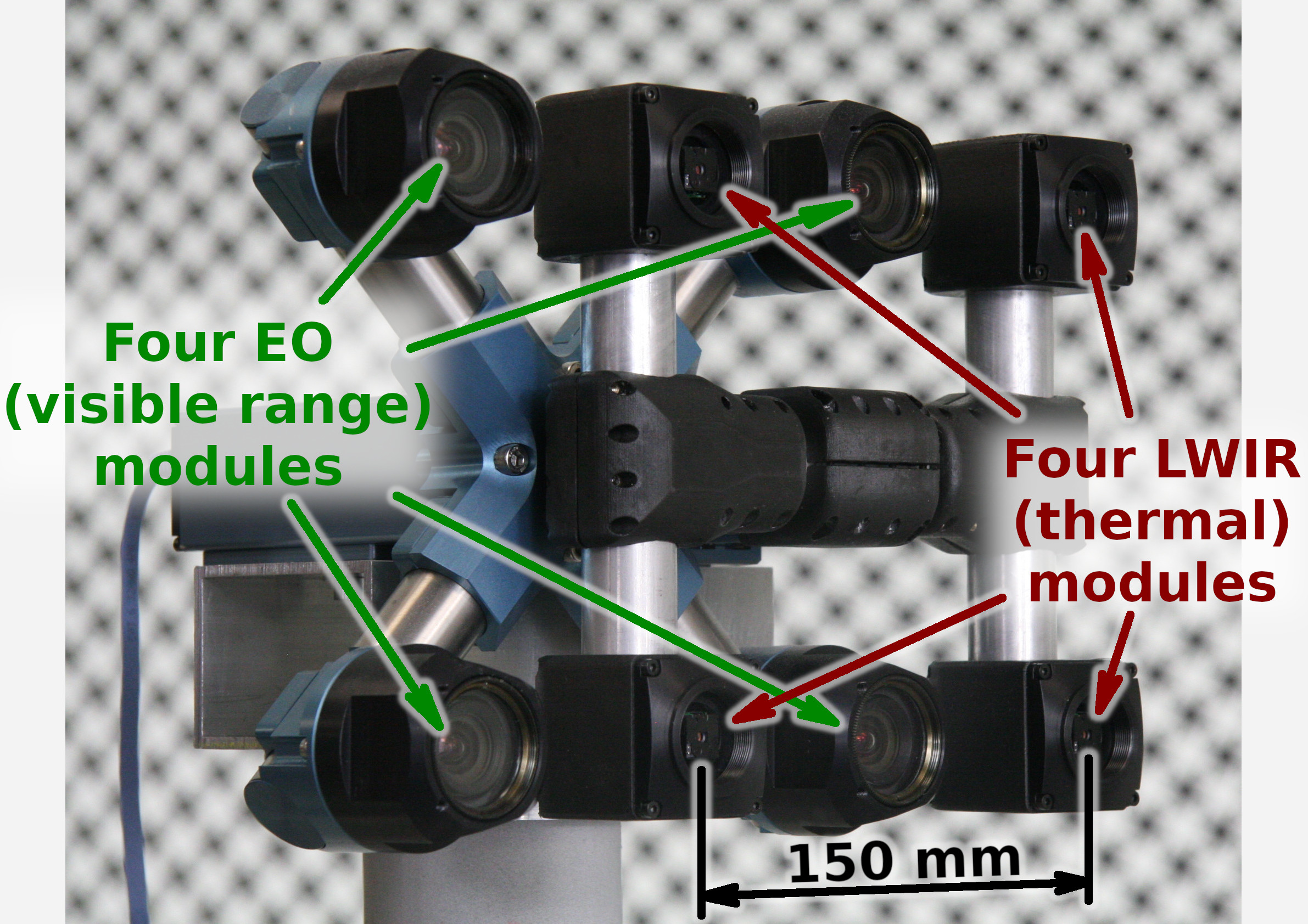
Figure 1. Talon (“instructor/student”) test camera.
Update: arXiv:1911.06975 paper about this project.
Summary
This post concludes the series of 3 publications dedicated to the progress of Elphel five-month project funded by a SBIR contract.
After developing and building the prototype camera shown in Figure 1, constructing the pattern for photogrammetric calibration of the thermal cameras (post1), updating the calibration software and calibrating the camera (post2) we recorded camera image sets and processed them offline to evaluate the result depth maps.
The four of the 5MPix visible range camera modules have over 14 times higher resolution than the Long Wavelength Infrared (LWIR) modules and we used the high resolution depth map as a ground truth for the LWIR modules.
Without machine learning (ML) we received average disparity error of 0.15 pix, trained Deep Neural Network (DNN) reduced the error to 0.077 pix (in both cases errors were calculated after removing 10% outliers, primarily caused by ambiguity on the borders between the foreground and background objects), Table 1 lists this data and provides links to the individual scene results.
For the 160×120 LWIR sensor resolution, 56° horizontal field of view (HFOV) and 150 mm baseline, disparity of one pixel corresponds to 21.4 meters. That means that at 27.8 meters this prototype camera distance error is 10%, proportionally lower for closer ranges. Use of the higher resolution sensors will scale these results – 640×480 and longer baseline of 200 mm (instead of the current 150 mm) will yield 10% accuracy at 150 meters, 56°HFOV.
(more…)
September 5, 2018
by Andrey Filippov
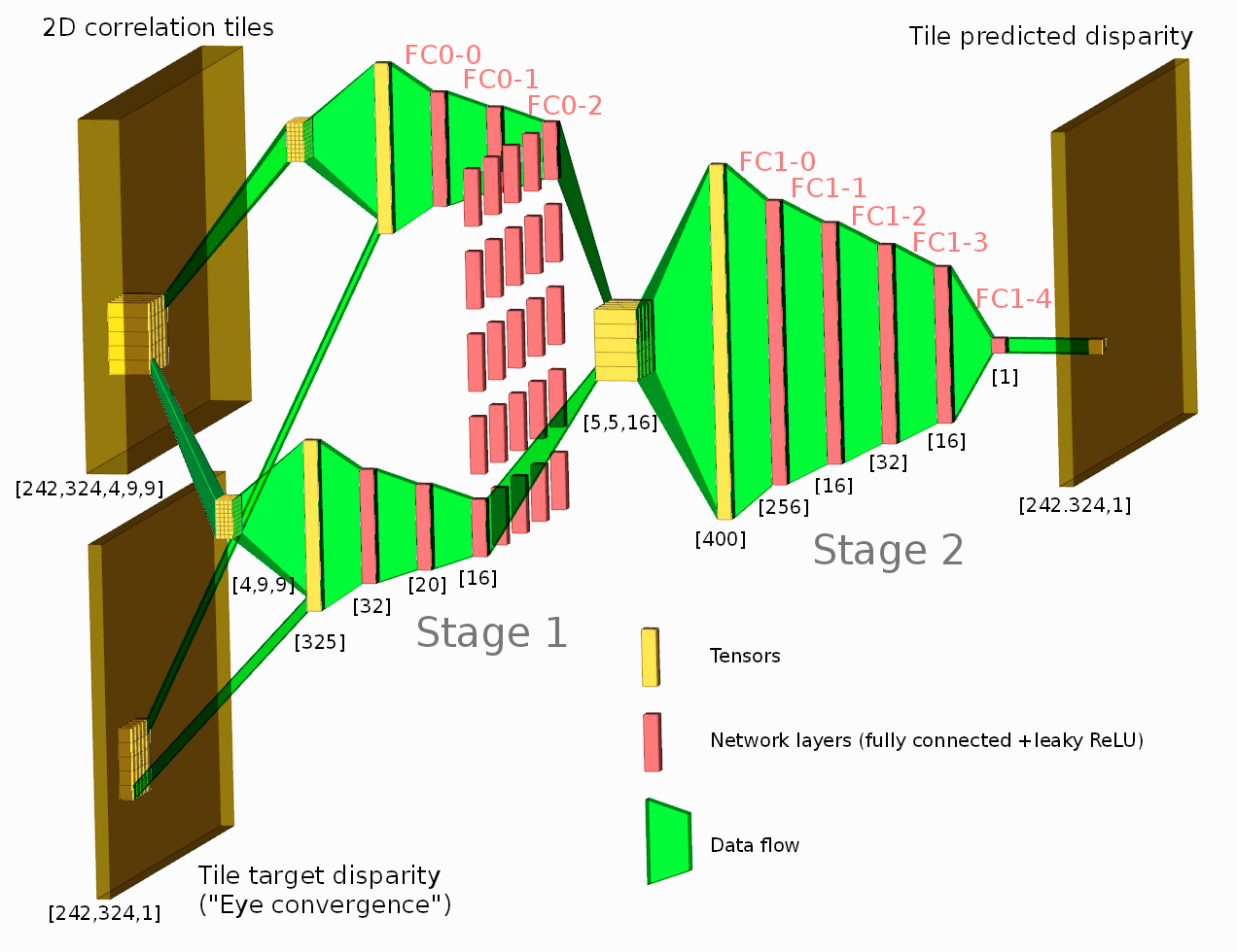
Figure 1. Network diagram. One of the tested configurations is shown.
Neural network connected to the output of the Tile Processor (TP) reduced the disparity error twice from the previously used heuristic algorithms. The TP corrects optical aberrations of the high resolution stereo images, rectifies images, and provides 2D correlation outputs that are space-invariant and so can be efficiently processed with the neural network.
What is unique in this project compared to other ML applications for image-based 3D reconstruction is that we deal with extremely long ranges (and still wide field of view), the disparity error reduction means 0.075 pix standard deviation down from 0.15 pix for 5 MPix images.
See also: arXiv:1811.08032
(more…)
May 6, 2018
by Andrey Filippov
Figure 1. Aircraft positions during descent captured with the quad stereo camera. Each animation frame corresponds to the available 3-D model.
While we continue to work on the multi-sensor stereo camera hardware (we plan to double the number of sensors to capture single-exposure HDR image sets) and develop code to get the ground truth data for the CNN training, we had some fun testing the camera for capturing aircraft position in 3-D space. Completely passive method, of course.
We found a suitable spot about 2.5 km from the beginning of the runway 34L of the Salt Lake City international airport (exact location is shown in the model viewer) so approaching aircraft would pass almost over our heads. With the 60°(H)×45°(V) field of view of the camera aircraft are visible when they are 270 m away horizontally.
(more…)
April 20, 2018
by Oleg Dzhimiev
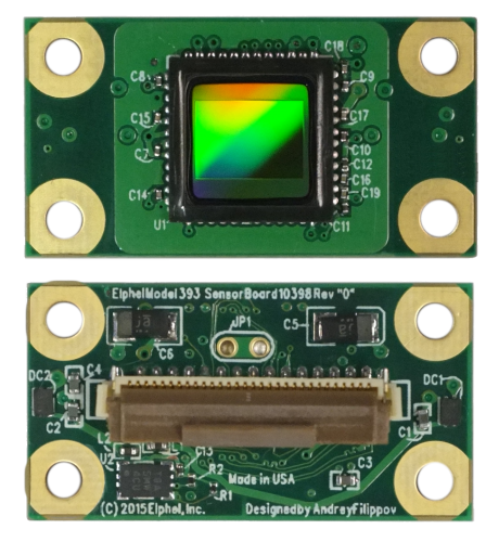
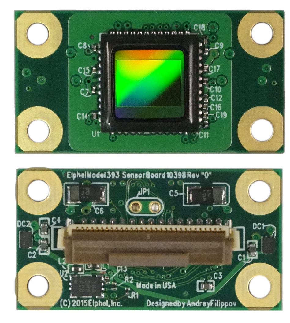
Fig.1 MT9F002
MT9F002
This post briefly covers implementation of a driver for On Semi’s MT9F002 14MPx image sensor for 10393 system boards – the steps are more or less general. The driver is included in the latest software/firmware image (
20180416). The implemented features are programmable:
- window size
- horizontal & vertical mirror
- color gains
- exposure
- fps and trigger-synced ports
- frame-based commands sequence allowing to change settings of any image up to 16 frames ahead (didn’t need to be implemented as it’s the common part of the driver for all sensors)
- auto cable phase adjustment during init for cables of various lengths
(more…)
March 20, 2018
by Andrey Filippov
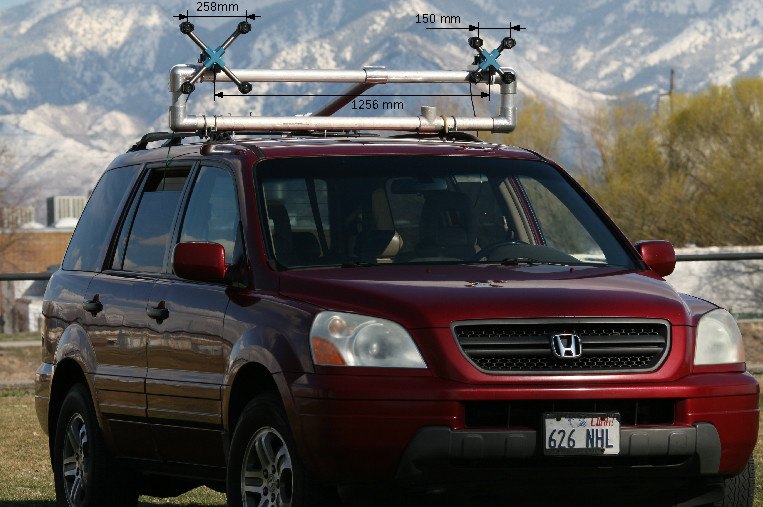
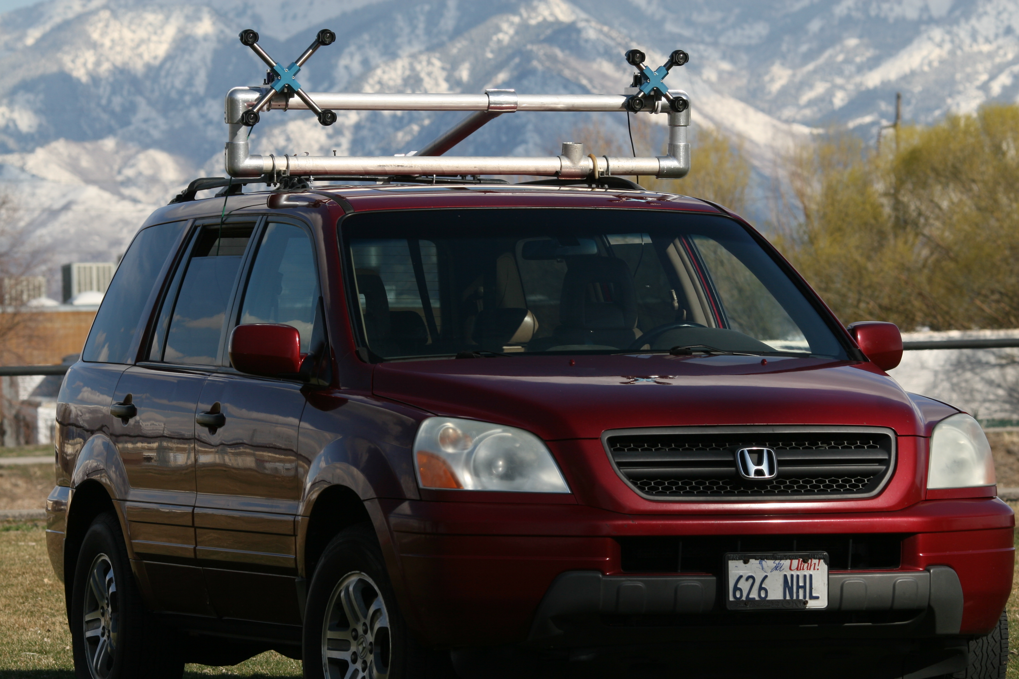
Figure 1. Dual quad-camera rig mounted on a car
Following the plan laid out in the earlier post we’ve built a camera rig for capturing training/testing image sets. The rig consists of the two quad cameras as shown in Figure 1. Four identical Sensor Front Ends (SFE) 10338E of each camera use 5 MPix MT9P006 image sensors, we will upgrade the cameras to 18 MPix SFE later this year, the circuit boards 103981 are in production now.
(more…)
February 5, 2018
by Andrey Filippov
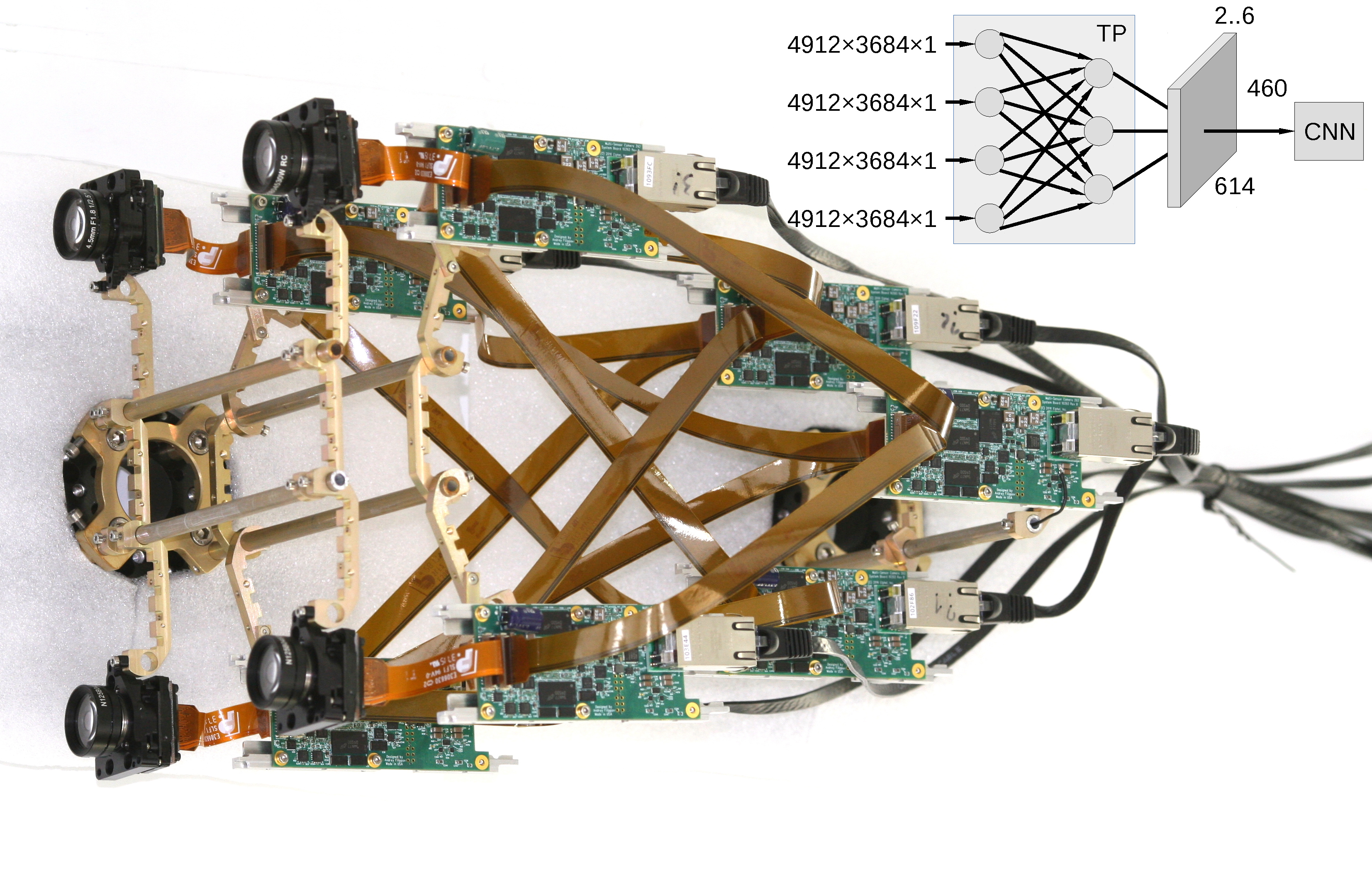
Figure 1. Multi-board setup for the TP+CNN prototype
Featured on Image Sensors World
This article describes our next steps that will continue the year-long research on high resolution multi-view stereo for long distance ranging and 3-D reconstruction. We plan to fuse the methods of high resolution images calibration and processing, already emulated functionality of the Tile Processor (TP), RTL code developed for its implementation and the Convolutional Neural Network (CNN). Compared to the CNN alone this approach promises over a hundred times reduction in the number of input features without sacrificing universality of the end-to-end processing. The TP part of the system is responsible for the high resolution aspects of the image acquisition (such as optical aberrations correction and image rectification), preserves deep sub-pixel super-resolution using efficient implementation of the 2-D linear transforms. Tile processor is free of any training, only a few hyperparameters define its operation, all the application-specific processing and “decision making” is delegated to the CNN.
(more…)
January 30, 2018
by Oleg Dzhimiev
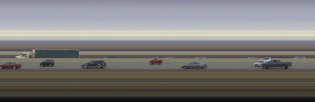
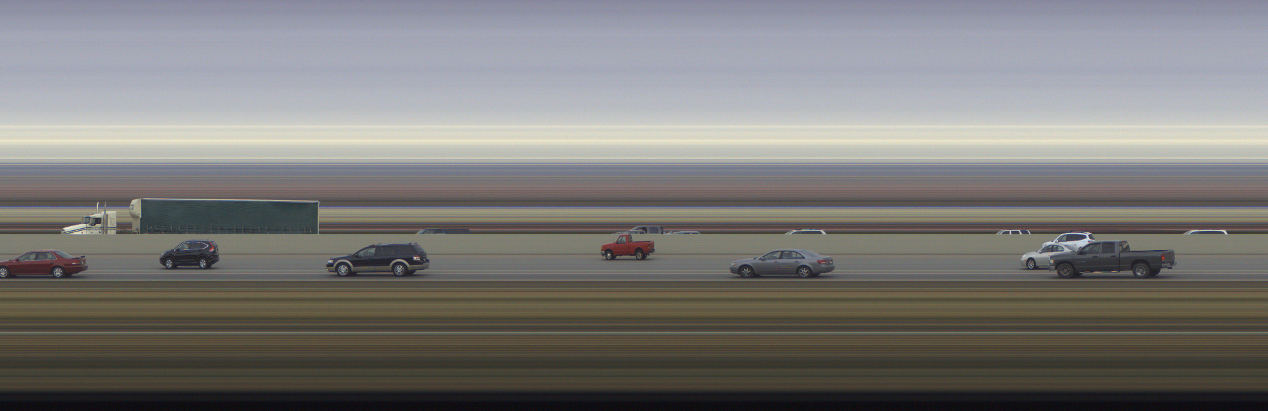
Photo Finish: all cars driving in the same direction effect
Since 2005 and the older 333 model, Elphel cameras have a Photo Finish mode. First, it was ported to 353 generation, and then from 353 to 393 camera systems.
In this mode the camera samples scan lines and delivers composite images as video frames. Due to the Bayer pattern of the sensor the minimal sample height is 2 lines. The max fps for the minimal sample height is 2300 line pairs per second. The max width of a composite frame can be up to 16384px (is determined by WOI_HEIGHT). A sequence of these frames can be simply joined together without any missing scan lines.
Current firmware (
20180130) includes a photo finish demo:
http://<camera_ip>/photofinish
A couple notes for 393 photo finish implementation:
- works in JP4 format (COLOR=5). Because in this format demosaicing is not done it does not require extra scan lines, which simplified fpga’s logic.
- fps is controlled:
- by exposure for the sensor in the freerun mode (TRIG=0, delivers max fps possible)
- by external or internal trigger period for the sensor in the snapshot mode (TRIG=4, a bit lower fps than in freerun)
See our wiki’s
Photo-finish article for instructions and examples.
January 8, 2018
by Andrey Filippov
This post continues discussion of the small tile space-variant frequency domain (FD) image processing in the camera, it demonstrates that modulated complex lapped transform (MCLT) of the Bayer mosaic color images requires almost 3 times less computational resources than that of the full RGB color data.
“Small Tile” and “Space Variant”
Why “small tile“? Most camera images have short (up to few pixels) correlation/mutual information span related to the acquisition system properties – optical aberrations cause a single scene object point influence a small area of the sensor pixels. When matching multiple images increase of the window size reduces the lateral (x,y) resolution, so many of the 3d reconstruction algorithms do not use any windows at all, and process every pixel individually. Other limitation on the window size comes from the fact that FD conversions (Fourier and similar) in Cartesian coordinates are shift-invariant, but are sensitive to scale and rotation mismatch. So targeting say 0.1 pixel disparity accuracy the scale mismatch should not cause error accumulation over window width exceeding that value. With 8×8 tiles (16×16 overlapped) acceptable scale mismatch (such as focal length variations) should be under 1%. That tolerance is reasonable, but it can not get much tighter.
What is “space variant“? One of the most universal operations performed in the FD is convolution (also related to correlation) that exploits convolution-multiplication property. Mathematically convolution applies the same operation to each of the points of the source data, so shifted object of the source image produces just a shifted result after convolution. In the physical world it is a close approximation, but not an exact one. Stars imaged by a telescope may have sharper images in the center, but more blurred in the peripheral areas. While close (angularly) stars produce almost the same shape images, the far ones do not. This does not invalidate convolution approach completely, but requires kernel to (smoothly) vary over the input images [1, 2], makes it a space-variant kernel.
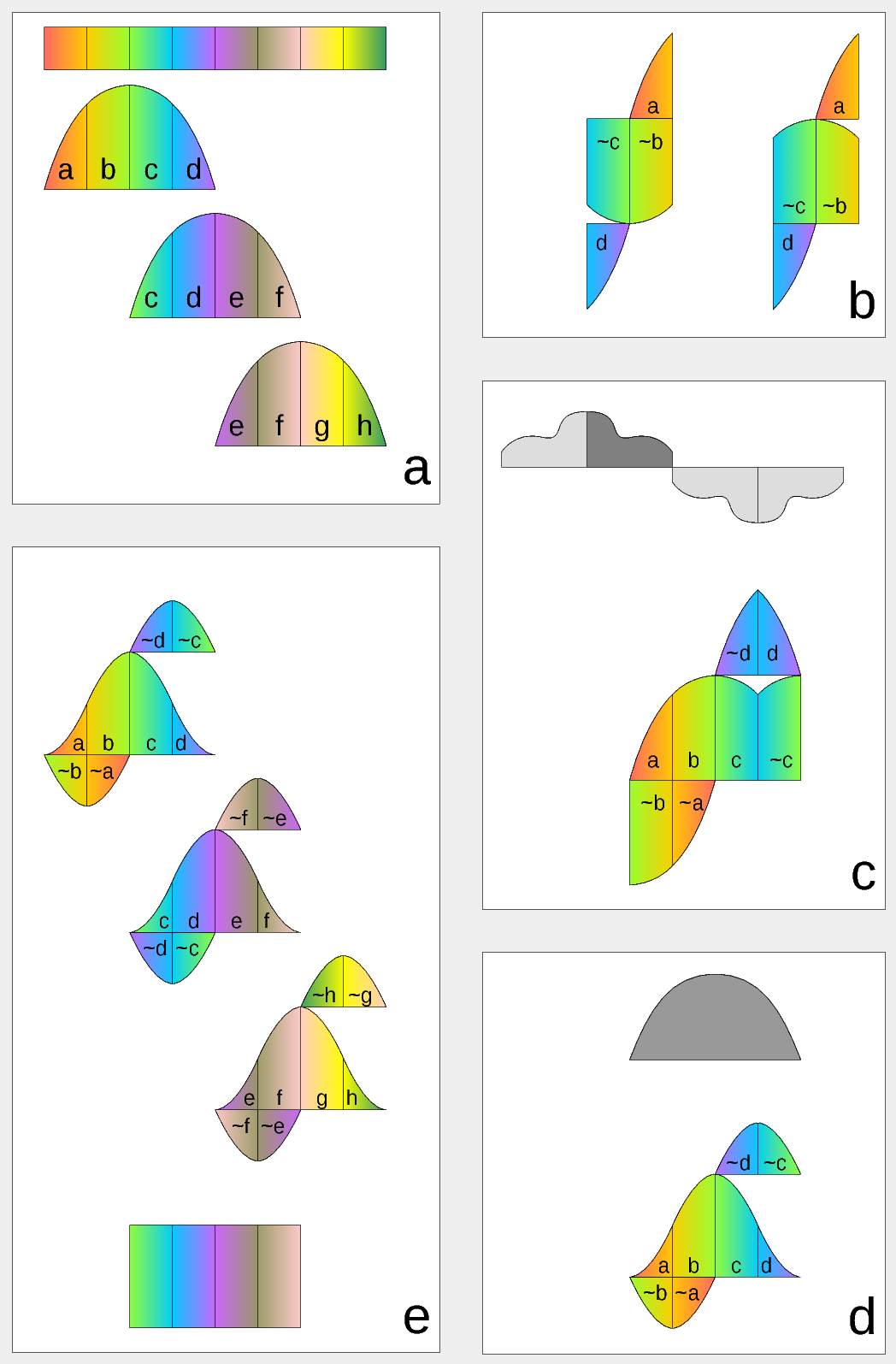
Figure 1. Complex Lapped Transform with DCT-IV/DST-IV: time-domain aliasing cancellation (TDAC) property. a) selection of overlapping input subsequences 2*N-long, multiplication by sine window; b) creating N-long sequences for DCT-IV (left) and DST-IV (right); c) (after frequency domain processing) extending N-long sequence using DCT-IV boundary conditions (DST-IV processing is similar); d) second multiplication by sine window; e) combining partial data
There is another issue related to the space-variant kernels. Fractional pixel shifts are required for multiple steps of the processing: aberration correction (obvious in the case of the lateral chromatic aberration), image rectification before matching that accounts for lens optical distortion, camera orientation mismatch and epipolar geometry transformations. Traditionally it is handled by the image rectification that involves re-sampling of the pixel values for a new grid using some type of the interpolation. This process distorts the signal data and introduces non-linear errors that reduce accuracy of the correlation, that is important for subpixel disparity measurements. Our approach completely eliminates resampling and combines integer pixel shift in the pixel domain and delegates the residual fractional pixel shift (±0.5 pix) to the FD, where it is implemented as a cosine/sine phase rotator. Multiple sources of the required pixel shift are combined for each tile, and then a single phase rotation is performed as a last step of pixel domain to FD conversion.
Frequency Domain Conversion with the Modulated Complex Lapped Transform
Modulated Complex Lapped Transform (MCLT)[3] can be used to split input sequence into overlapping fractions, processed separately and then recombined without block artifacts. Popular application is the signal compression where “processed separately” means compressed by the encoder (may be lossy) and then reconstructed by the decoder. MCLT is similar to the MDCT that is implemented with DCT-IV, but it additionally preserves and allows frequency domain modification of the signal phase. This feature is required for our application (fractional pixel shifts and asymmetrical lens aberrations modify phase), and MCLT includes both MDCT and MDST (that use DCT-IV and DST-IV respectively). For the image processing (2d conversion) four sub-transforms are needed:
- horizontal DCT-IV followed by vertical DCT-IV
- horizontal DST-IV followed by vertical DCT-IV
- horizontal DCT-IV followed by vertical DST-IV
- horizontal DST-IV followed by vertical DST-IV
(more…)
Next Page »