TPNET with LWIR
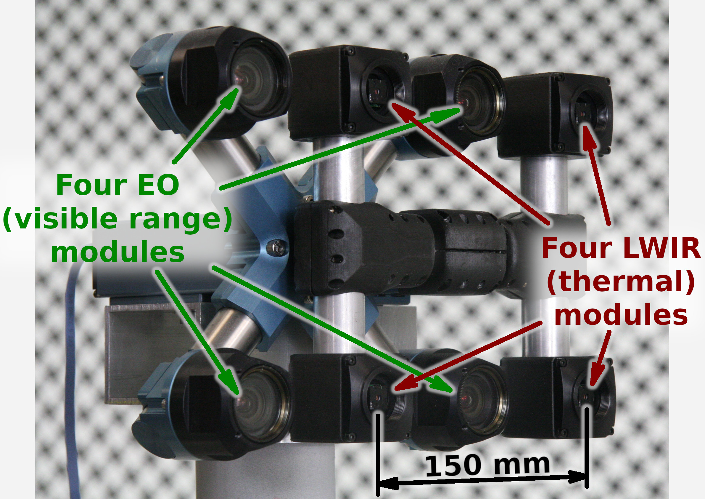
Figure 1. Talon (“instructor/student”) test camera.
Contents
Update: arXiv:1911.06975 paper about this project.
Summary
This post concludes the series of 3 publications dedicated to the progress of Elphel five-month project funded by a SBIR contract.
After developing and building the prototype camera shown in Figure 1, constructing the pattern for photogrammetric calibration of the thermal cameras (post1), updating the calibration software and calibrating the camera (post2) we recorded camera image sets and processed them offline to evaluate the result depth maps.
The four of the 5MPix visible range camera modules have over 14 times higher resolution than the Long Wavelength Infrared (LWIR) modules and we used the high resolution depth map as a ground truth for the LWIR modules.
Without machine learning (ML) we received average disparity error of 0.15 pix, trained Deep Neural Network (DNN) reduced the error to 0.077 pix (in both cases errors were calculated after removing 10% outliers, primarily caused by ambiguity on the borders between the foreground and background objects), Table 1 lists this data and provides links to the individual scene results.
For the 160×120 LWIR sensor resolution, 56° horizontal field of view (HFOV) and 150 mm baseline, disparity of one pixel corresponds to 21.4 meters. That means that at 27.8 meters this prototype camera distance error is 10%, proportionally lower for closer ranges. Use of the higher resolution sensors will scale these results – 640×480 and longer baseline of 200 mm (instead of the current 150 mm) will yield 10% accuracy at 150 meters, 56°HFOV.
| # | Scene timestamp and comments [Expand all] | Non-TPNET disparity error (pix) | TPNET disparity error (pix) | TPNET accuracy gain | ||||||||||||||||||||||||||||||||||||||
|---|---|---|---|---|---|---|---|---|---|---|---|---|---|---|---|---|---|---|---|---|---|---|---|---|---|---|---|---|---|---|---|---|---|---|---|---|---|---|---|---|---|---|
| 1 | 1562390202_933097: Single person, trees.
|
0.136 | 0.060 | 2.26 | ||||||||||||||||||||||||||||||||||||||
| 2 | 1562390225_269784: Single person, trees.
|
0.147 | 0.065 | 2.25 | ||||||||||||||||||||||||||||||||||||||
| 3 | 1562390225_839538: Single person. Horizontal motion blur.
|
0.196 | 0.105 | 1.86 | ||||||||||||||||||||||||||||||||||||||
| 4 | 1562390243_047919: No people, trees.
|
0.136 | 0.060 | 2.26 | ||||||||||||||||||||||||||||||||||||||
| 5 | 1562390251_025390: Open space. Horizontal motion blur.
|
0.152 | 0.074 | 2.06 | ||||||||||||||||||||||||||||||||||||||
| 6 | 1562390257_977146: Three persons, trees.
|
0.146 | 0.074 | 1.96 | ||||||||||||||||||||||||||||||||||||||
| 7 | 1562390260_370347: Three persons, near and far trees, minivan.
|
0.122 | 0.058 | 2.12 | ||||||||||||||||||||||||||||||||||||||
| 8 | 1562390260_940102: Three persons, trees.
|
0.135 | 0.064 | 2.12 | ||||||||||||||||||||||||||||||||||||||
| 9 | 1562390317_693673: Two persons, far trees.
|
0.157 | 0.078 | 2.02 | ||||||||||||||||||||||||||||||||||||||
| 10 | 1562390318_833313: Two persons, trees.
|
0.136 | 0.065 | 2.10 | ||||||||||||||||||||||||||||||||||||||
| 11 | 1562390326_354823: Two persons, trees.
|
0.144 | 0.090 | 1.60 | ||||||||||||||||||||||||||||||||||||||
| 12 | 1562390331_483132: Two persons, trees.
|
0.209 | 0.100 | 2.08 | ||||||||||||||||||||||||||||||||||||||
| 13 | 1562390333_192523: Single person, sun-heated highway fill.
|
0.153 | 0.067 | 2.30 | ||||||||||||||||||||||||||||||||||||||
| 14 | 1562390402_254007: Car on a highway, background trees.
|
0.140 | 0.077 | 1.83 | ||||||||||||||||||||||||||||||||||||||
| 15 | 1562390407_382326: Car on a highway, background trees.
|
0.130 | 0.065 | 2.01 | ||||||||||||||||||||||||||||||||||||||
| 16 | 1562390409_661607: Single person, a car on a highway.
|
0.113 | 0.063 | 1.79 | ||||||||||||||||||||||||||||||||||||||
| 17 | 1562390435_873048: Single person, two parked cars.
|
0.153 | 0.057 | 2.68 | ||||||||||||||||||||||||||||||||||||||
| 18 | 1562390456_842237: Close trees.
|
0.211 | 0.102 | 2.08 | ||||||||||||||||||||||||||||||||||||||
| 19 | 1562390460_261151: Trees closer than the near clipping plane.
|
0.201 | 0.140 | 1.44 | ||||||||||||||||||||||||||||||||||||||
| Average | 0.154 | 0.077 | 2.04 | |||||||||||||||||||||||||||||||||||||||
Notes: click on the scene title to show details. Click on the image to start/stop GIF animation.
Detailed results
Figure 2 illustrates results at the output and at the intermediate processing steps. Similar data is availble for each of the 19 evaluated scenes listed in the Table 1 (Figure 2 corresponds to scene 7, highlighted in the table).
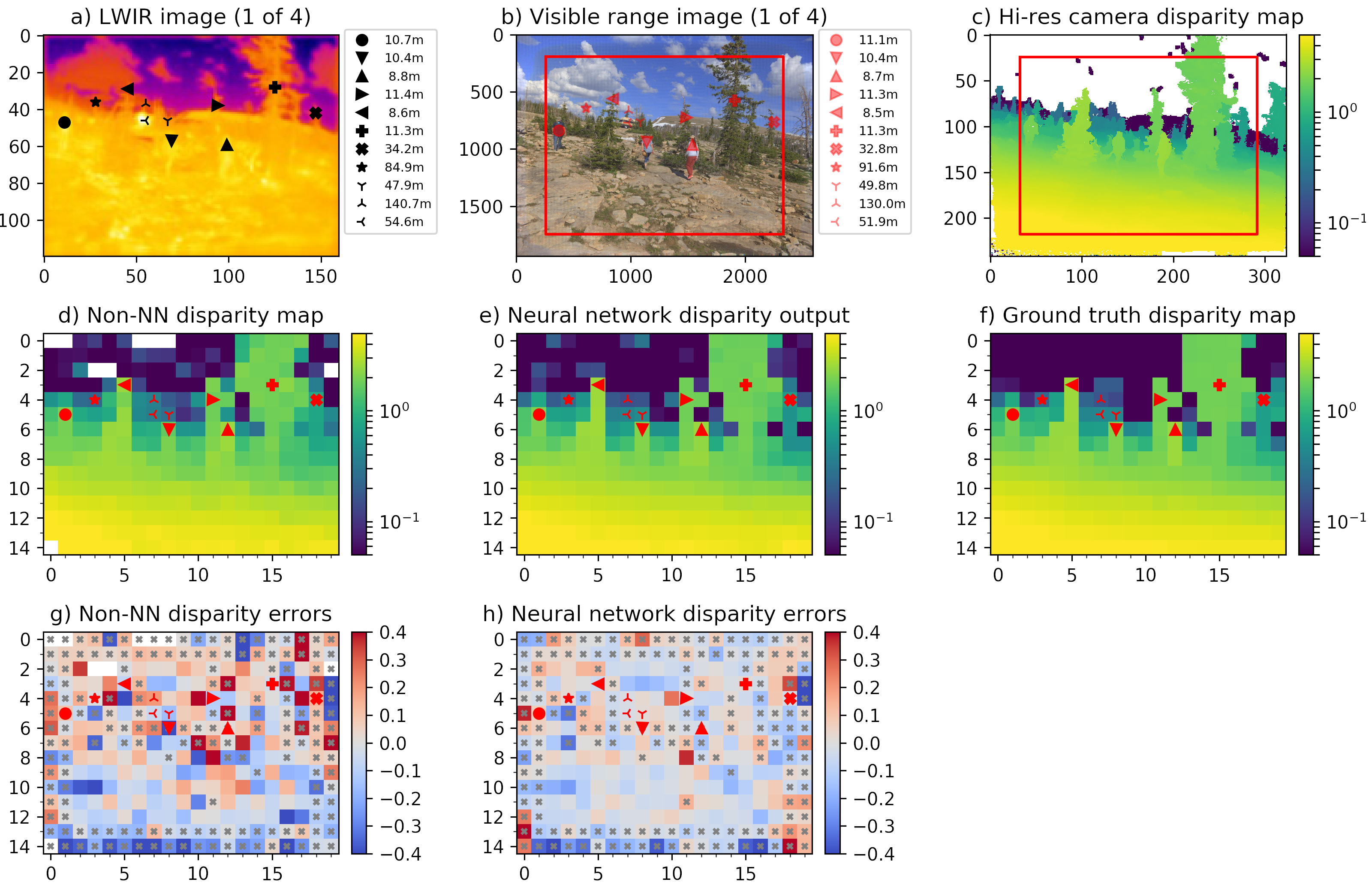
Figure 2. LWIR depth map generation and comparison to the ground truth data.
Processing steps to generate and evaluate LWIR depth maps
Four visible range 5 Mpix (2592×1936) images (Figure 2b) are corrected from the optical aberrations and are used to generate disparity map c) that has 1/8 resolution (324×242 where each pixel corresponds to an overlapping 16×16 tile in the source images) with the Tile Processor. Red frames in b) and c) indicate field of view of the LWIR camera modules. Each of the high resolution disparity tiles in c) is mapped to the corresponding tiles of the 20×15 LWIR disparity map f). This data is used as ground truth for both neural network training and subsequent testing and inference (20% of the captured 1100 image sets are reserved for testing, 80% are used for training).
One of the 4 simultaneously acquired LWIR images is shown in Figure 2a. Table 1 contains animated GIFs for each set of 4 scene images, animation (click image to start) consequently shows all 4 views of the quad camera setup. These 4 LWIR images are partially rectified and then subject to 2D correlation between each of the 6 image pairs, resulting in the disparity map d) similarly to how it is done for the visible range (aka electro-optical or EO) ones. Sub-plot g) shows the difference between LWIR disparity map calculated without machine learning d) and the ground truth data f). Subplot e) contains disparity map enhanced by the ML that uses raw 2D-correlation data (Figures 3, 4) as its input features. And the last subplot h) shows difference between e) and f) as the resudual errors after full TPNET processing. Manually placed markers listed in a) and b) correspond to the scene features, black markers in a) show linear distances calculated from the output e), while red markers legend in b) lists the corresponding ground truth distances. Table 1 contain the same data and additionally shows relative errors of the LWIR measurements.
Gray “×”-es in g) and h) indicate tiles where data may be less reliable. These tiles include 2-tile margins on each side of the map, caused by the fact that convolution part of the neural network analyses 5×5 tile clusters. Bottom edge tiles use pixels that are not available in top pair of the four images because of the large parallax for the near objects, so bottom tiles use only a single binocular pair instead of the 6 available for the inner tiles.
Another case of the potential mismatch between the disparity output and the ground truth data is when different range objects in high-resolition map c) correspond to the same tile in LWIR maps d) and e). The network is trained to avoid averaging of the far and near objects in the same tile, but it still can wrongly identify which of the planes (foreground or background) was selected for the ground truth map. For this reason all LWIR tiles that have both foreground and background match in c) are also marked.
Most of the tiles that have both foreground and background objects are assigned corectly so we do not remove the marked tiles from the average error calculation. Instead we handle gross outliers by discarding a fixed fraction of all tiles (we used 10%) that have the largest disparity errors and average errors among the remaining 90% of tiles.
Depth maps X/Y resolution
Disparity maps generated from the low resolution 160×120 LWIR sensors of the prototype camera have even lower resolution of just 20×15 tiles. There are other algorithms that generate depth maps with the same pixel resolution as the original images, but they have lower ranging accuracy. Instead we plan to fuse high-reolution (pixel-accurate) rectified source images and low X/Y (but high Z) resolution depth maps with another DNN. That was not a part of this project, but it is doable — similar approach is already used for fusion of the high-resolution regular images with the low pixel resolution time-of-flight (ToF) cameras or LIDARs. Deep subpixel resolution needed for the ranging accuracy requires many participating pixels for each object no be measured, so the fusion will not significantly increase the number of different objects in each tile, but it can restore the pixel accuracy of the object contours.
Comments on the individual scenes
Among the evaluated scenes there are two with strong horizontal motion blur caused by the operator turning around the vertical axis – scenes 3 and 5. Such blur can not be completely eliminated by the nature of the microbolometer sensors, so the 3D perception has to be able to mitigate it. If it was just a traditional binocular system, horizontal blur would drown useful data in the noise and make it impossible to achieve a deep subpixl resolution. Quad non-colinear stereo layout is able to mitigate this problem and the acuracy drop is less prominent.
The last two scenes (18 and especially 19) demonstrate high disparity errors (0.1 and 0.14 pixels respectively). These large errors correspond to high absolute disparity value (over 8 pix) and low distances (under 3 meters) where disparity variations within the same tile are high and so the disparity of a tile is ambiguous. On the other hand, relative disparity error for even 0.4 pixels is only 5% or just 15 cm at 3 m range. Scene 19 has details in the right side that are closer than the near clipping plane preset for of the ground truth camera.
TPNET – Tile Processor with the deep neural network
Image rectification and 2D correlation
Earlier post “Neural network doubled effective baseline of the stereo camera” (and also arXiv:1811.08032 preprint) explains the process of aberration correction, partial rectification of the source images and calcualtion of the 2D phase correlation using Complex Lapped Transform (CLT) for the 16×16 overlapping tiles (stride 8) of the quad camera high resolution visible range images. We used the same algorithms in the current project too. Depth perception with TPNET is a 2-step process (actually iterative as these steps may need be repeated) similar to the human stereo vision – first the eyes are converged at the objects at certain distance producing zero disparity between the two images there, then data from the pair of images is processed (locally in retinas and then in the visual cortex) to extract residual mismatch and convert it to depth. There are no moving parts in TPNET-based system, instead the Tile Processor implements target disparity (“eye convergence”) by image tile shifts in the frequency domain with CLT, so it is as if each of the image tiles had a set of 4 small “eyes” that simultaneously can converge at different distances.
Figure 3. Set of four images of the scene 7. (click to start/stop)
Figure 3 shows partially rectified set of 4 LWIR images of the scene 7. “Partially” means that they are not rectified to the complete rectilinear (pinhole) projection, but are rather subject to subtle shifts to a common to all four of them radial distortion model. CLT is similar to 2D Fourier transform and is also invariant to shifts, but not to stretches and rotations. We use subpixel-accurate tile shifts in the frequency domain, benefitting from the fact that individual lenses while different have similar focal length and distortion parameters. Complete distortion correction would require image resampling increasing computation load and memory footprint or reducing subpixel resolution.
Next two figures contain 2D phase correlation data that is fed to the DNN part of TPNET. Figure 4 is calculated with each tile target disparity of zero (converged at infinity). The four frames of the GIF animation correspond to 4 stereo pairs directions – horizontal, vertical and 2 diagonals, as indicated in the top left image corner.
 Figure 4. 2D phase correlations with all tiles target disparity set to 0. (click to start/stop) |
 Figure 5. 2D phase correlations, target disparity set by the polynomial approximaton. (click to start/stop) |
Similarly to the source images (Figure 3) all the correlation tiles for infinity objects (as clouds in the sky) do not move when animation is running, while the near objects do – the residual disparity (diffenece beween the full disparity and the “target disparity”) value corresponds to the offest of the spot center from the grid center in the dirrection of the red arrows. The correlation result is most accurate when residual disparity is near zero, the farther the spot center is from zero, the less source pixels participate in matching and so the correlation S/N ratio and resolution drop.
Figure 5 is similar, but this time each tile target disparity is set by the iterative process of finding residual correlation argmax by the polynomial approximation and re-calculating new 2D correlation. This time most of the tiles do not move, except those that are on the foreground/backgroud boreders.
Neural network layout
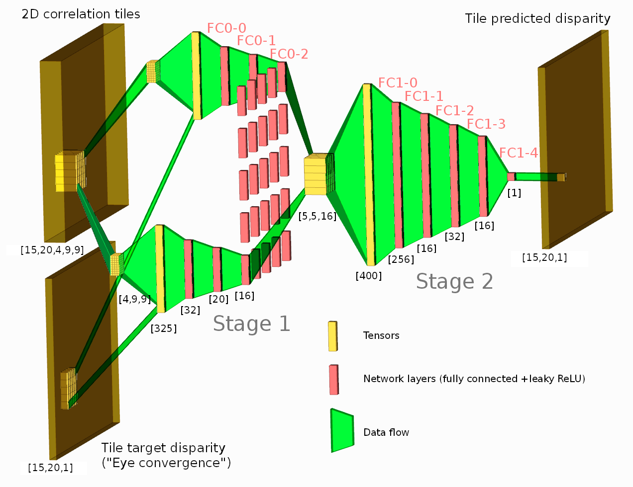
Figure 6. Network diagram
The 2D phase correlation tiles shown above and the per-tile target disparity value make the input features that are fed to the neural network during training and later inference. We tried the same network architecture and cost finctions we developed for the high resolution cameras (blog post, arXiv:1811.08032 preprint) and it behaved really well, allowing us to finish this project in time.
The network consists of two stages, where the first one gets input features from a single tile 2D phase correlation as [4,9,9] tensor (first dimension, 4 is the number of correlation pairs, two others (9×9) specify the center window of the full 15×15 2D correlation – 4 pixels in each direction around the center). Stage 1 output for each tile is a 16-element vector fed to the Stage 2 inputs.
Stage 2 subnet for each tile gets input features from the corresponding stage 1 output and its 24 neighbors in a form of a [5,5,16] tensor. The output of the stage 2 is a single scalar for each tile or [15,20,1] tensor for the whole disparity map, shown in Figure 2e. Such two-stage layout is selected to allow the network to use neighbor tiles when generating its disparity output (such as to continue edges, to fill low-textured areas, and to improve foreground/background separation), but simultaneously limit dimensions of the fully connected layers.
Training and the cost function
Instead of the full images the training sets consist of the 5×5 tile fragments harvested from the 880 image sets. Randomly constructed batches use 2D histogram normalization of the image tiles, so each batch includes similar repesenation of near and far, high contrast and low contrast tiles. Cost function design followed the same approach as described in the earlier post, we clipped the L2 cost of the difference with ground truth (essentially giving up on gross outliers caused by incorrect foreground/background tiles assignment) and included additional terms.
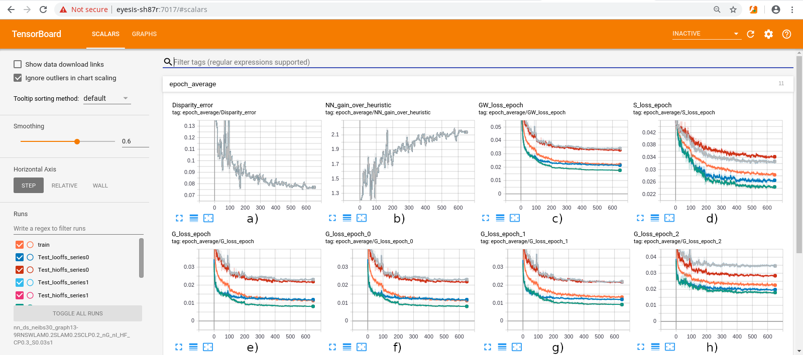
Figure 7. Screenshot of the Tensorboard after TPNET training. a) test image average disparity error; b) network accuracy gain over heuristic (non-NN); c) total cost function; d) cost of “cutting corners” between the foreground and background; e) cost of mixture of L2 for 5×5, 3×3 and single tile Stage2; f) cost for 5×5 only (used for inference); g) cost for 3×3 only; h) cost for single tile only.
Additional cost function terms included regularization to reduce overfitting, and the one to avoid averaging of the distances to the foreground and background objects for the same tile, forcing the network to select either fore- or background, but not their mixture.
Regularization included “shortcuts” requiring that if just a single (center) tile input from Stage 1 is fed to stage 2, it should provide less accurate but still reasonably good disparity output (Figure 7h), same for the 3×3 sub-window (Figure 7g). Only full 5×5 Stage 2 output (Figure 7f) is used for test image evaluation and inference, but training uses a weighted mixture of all three (Figure 7e).
Cost function term to reduce averaging of foreground and background disparities in the border tiles (Figure 7d) is made in the following way: for each tile the average of the ground truth disparities of its 8 neighbors is calculated, and additional cost is imposed if the network output falls between the ground truth and this average. Figure 7c shows the total cost function that combines all individual terms.
Conclusion
- Experiments with the prototype LWIR 3D camera provided disparity accuracy consistent with our earlier results obtained with the high resolution visible range cameras.
- The new photogrammetric calibration pattern design is adequate for the LWIR imaging and can be used for factory calibration of the LWIR cameras and camera cores.
- Machine learning with TPNET provided 2× ranging accuracy improvement over the one obtained with the same data and traditional only (w/o machine learning) processing.
- Combined results proved the feasibility of completely passive LWIR 3D perception even with relatively low resolution thermal sensors.
Leave a Reply