Two Dimensional Phase Correlation as Neural Network Input for 3D Imaging
We uploaded an image set with 2D correlation data together with the import Python code for experiments with the neural networks and are now looking for collaboration with those who would love to apply their DL experience to the new kind of input data. More data will follow and we welcome feedback to make this data set more useful.
The application area we are interested in is an extremely long distance 3D scene reconstruction and ranging with the distance to baseline ratio of 1000:1 to 10,000:1 while preserving wide field of view. Earlier post describes aircraft distance and velocity measurements with up to 3,000:1 distance-to-baseline ratio and 60°(H)×45°(V) field of view.
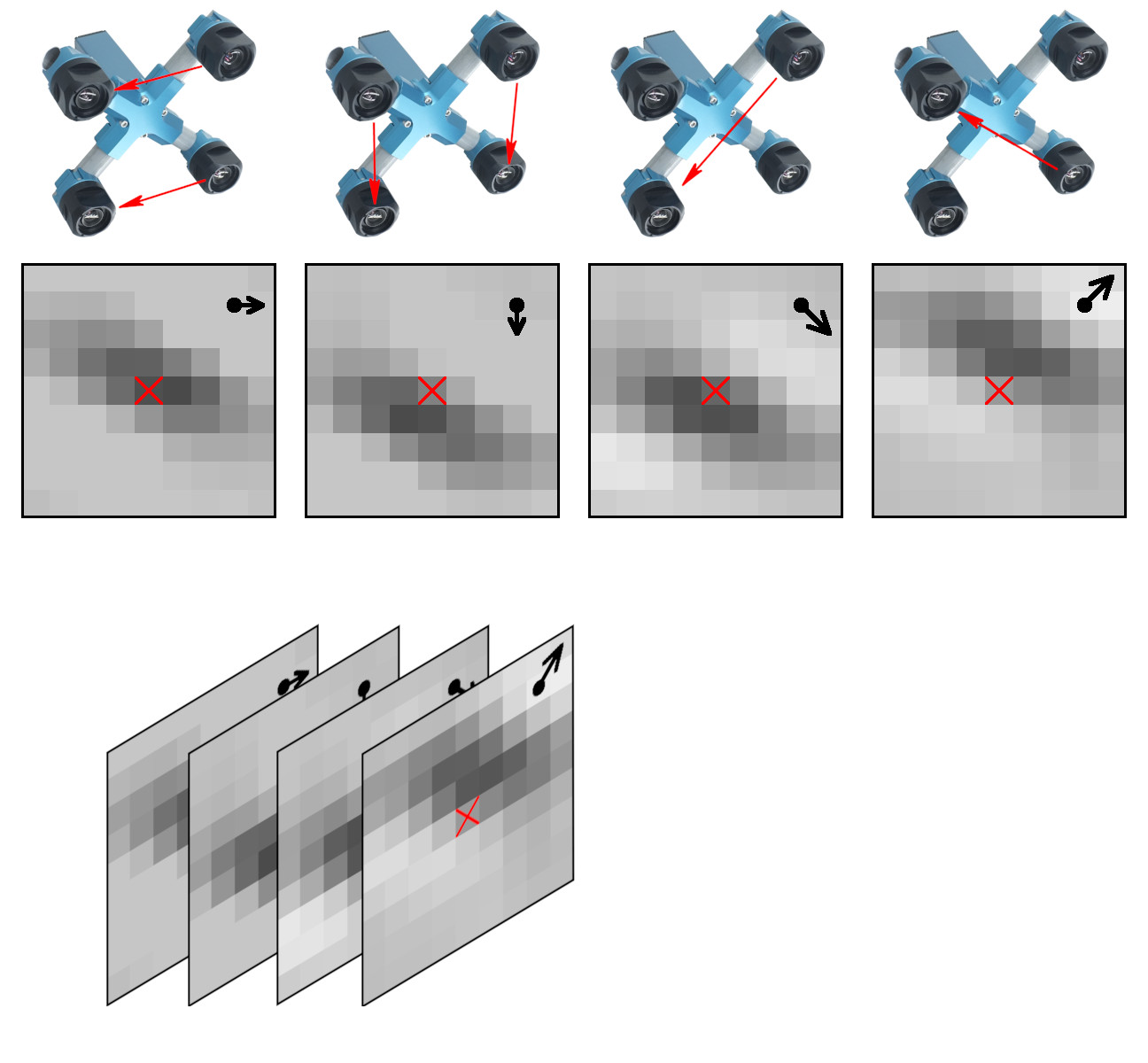
Figure 1. Space-invariant 2D phase correlation data
Contents
Data set: source images, 2D correlation tiles, and X3D scene models
The data set contains 2D phase correlation output calculated from the 2592×1936 Bayer mosaic source images captured by the quad stereo camera, and Disparity Space Image (DSI) calculated from a pair of such cameras. Longer baseline provides higher range resolution and this DSI is serving as the ground truth for a single quad camera. The source images as well as all the used software is also provided under the GNU/GPLv3 license. DSI is organized as a 324×242 array – each sample is calculated from the corresponding 16×16 tile. Tiles are overlapping (as shown in Figure 3) with stride 8.
These data sets are provided together with the fully reconstructed X3D scene models, viewable in the browser (Wavefront OBJ files are also generated). The scene models are different from the raw DSI as the next software stages generate meshes, and that frequently leads to over-simplification of the original DSI (so most fronto parallel objects in the scene provide better range accuracy when probed near the bottom). Each scene is accompanied with the multi-layer TIFF file (*-DSI_COMBO.tiff) that allows to see the difference between the measured DSI and the one used in the rendered X3D model. File format and Python import software is documented in Oleg’s post “Reading quad stereo TIFF image stacks in Python and formatting data for TensorFlow”, the data files are directly viewable with ImageJ.
The first goal of applying neural network to this data is to improve DSI generation from the raw 2D correlation compared to what we can do now with the traditional code by using data from all correlation pairs and the neighbor tiles to propagate information along the objects edges and amplify correlation in low textured areas by pooling the correlation outputs from multiple tiles.
While there are no moving parts in the system, the overall process of measuring the DSI resembles human/animal stereo vision, where the eyes are converged for the expected object distance, and the visual processing deals with only a small residual mismatch, constantly adjusting the convergence. The difference here is that each tile can be individually “converged” for the requested disparity – this is done by combining integer pixel shift of the tile input window with the accurate fractional pixel shift by a phase rotator in the frequency domain to avoid any re-sampling errors. Currently prediction of the “convergence” (expected disparity) for the next tiles to measure is performed by a mixture of several algorithms (to avoid an expensive full disparity scan over the whole image). This process of predicting disparity is likely to be improved by a properly designed and trained network too, the one that will use the tile context.
As the current processing is recurrent (repeated “eye convergence” / mismatch processing), there are several options how to organize the training data. We decided to focus on sub-pixel matching, so for each scene with calculated ground truth DSI (from the dual camera rig) the correlation output is measured for the target disparity (convergence) in the range of minus 1 pixel to plus 1 pixel with the step of 0.1 pixel in the currently provided data sets. It makes total of 21 files of the correlation outputs. This partial disparity sweep around the ground truth is an alternative to a full disparity sweep that would require too much storage.
In addition to the raw Bayer images scene models have links to the JPEG images, corresponding to each sub-camera view. These images have aberrations corrected and they are partially rectified for the disparity = 0 (infinity). They are not rectilinear, and still have small radial distortion common to all of them, it is compensated during generation of the x3d models. The images have visible modulation caused by the Bayer mosaic – they were not subject to any (destructive) demosaic processing – only to the linear one. Each color channel is separately de-convolved with a set of space-variant kernels.

Figure 2. Dual quad camera rig
Available data series
Initial data contains scenes captured with the car mounted dual quad camera rig (Figure 2) in two series:
- Salt Lake City State Street ↗
- Salt Lake City overlook (northern part of the city in the direction of the airport) ↗
- Airliner approaching SLC International airport ↗
The first series (80 scenes) was captured while driving north at a rate of 5 frames per second. Only the first four seconds (20 scenes) of each 20 second interval are posted to reduce the amount of uploaded data. The second series (59 scenes) was captured while standing and then slowly turning and starting to move. Third series was made from the stationary camera pointed in the direction of the airport.
More data will be added, we are open to suggestions – what data should be included to make the whole data set more useful. All available series combined are available at this link: ↗. Number of the scenes is definitely too small to extract the semantic information, but it may be enough to train the network to build DSI using small samples of the correlation tiles. At least to start with.
The frequently asked questions about this dataset
Why is there a special format of the data set, why not just provide the raw images?
We do provide raw Bayer images captured by the camera in JP4 format, but due to significant for the high-resolution images optical aberrations, complete end-to-end processing would require space-variant coefficients that to our understanding would require enormous resources and a very large number of images for training. Instead we propose to separate the space-variant pre-processing and provide space-invariant data to the network. And the 2D correlation data is the earliest space-invariant data available with this approach.
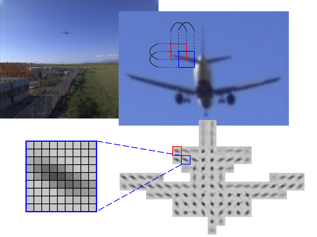
Figure 3. Anisotropy of the 2D correlation. Red and blue squares show two overlapping tiles in the source images and in the calculated 2D correlation.
Why do you use four cameras for stereo when most systems have just two?
In the case when the source image contains nicely textured in all directions areas, the correlation output contains a sharp round spot and subpixel argmax calculation is not very difficult – polynomial interpolation provides good results. Unfortunately many real-life objects do not have convenient texture, and poor texture is Achilles’ heel of many vision-based 3D reconstruction systems. On the other hand discontinuity between foreground and background objects usually results in sharp edges that can be used for matching, and it is usually safe to assume that lack of visible features means that the surface is smooth and depth can be reconstructed by averaging over larger area. The edges may have any direction, but binocular systems with horizontal baselines are only sensitive to the vertical features. Figure 3. shows correlation output of a distant airplane where the correlation spots are stretched in the direction of the edges. The four-sensor camera in Figure 1 contains 6 pairs, and after combining horizontal and vertical there are 4 directions left, so for any edge direction there is a pair with a almost perpendicular to it.
Why don’t you use LIDARs for the ground truth data?
Most available LIDARs have a rather short range of 150-250 meters, and we are interested in measuring larger scenes. So instead we decided to use a pair of similar quad cameras positioned at ~5 times larger distance than the quad camera baseline, so the measurements it provides are also 5 times more accurate and can be used for training as ground truth. Binocular system does have limitations as described above, so it will not provide accurate data for the horizontal features (like electrical wires so common over Salt Lake City).
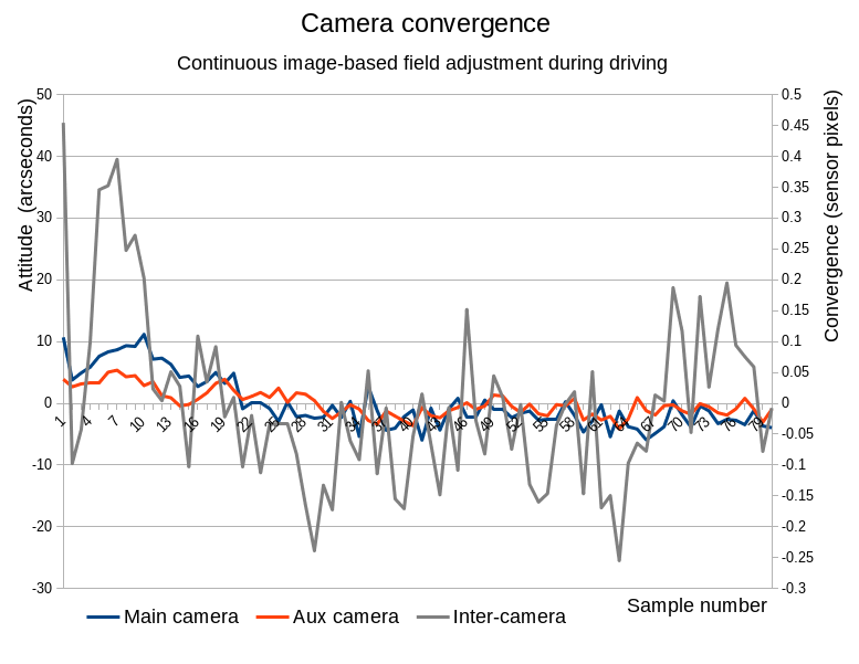
Figure 4. Field calibration results
What are the current limitations of the hardware?
Individual quad cameras use precisely thermally compensated sensor front ends with the image plane movement relative to the sensor of less than ±0.02μ/°C, but the overall mount made of titanium tubes does bend when heated by the sun radiation from one side. Just few tenths of a pixel, but it is too much for the application, so until we have a new design we have to use field calibration and bundle-adjust individual sub-camera attitudes using the image data itself. It allows to keep misalignment to ~0.05 pix.
Dual camera rig (Figure 2) as currently implemented has its limitations that we temporarily mitigate with the field calibration. We are working on the rig improvements too – one of the mechanical issues is that when driving at freeway speeds we noticed 55 Hz torsion oscillations (two cameras rotating in opposite directions at the ends of the 1.5 m aluminum tube) of 0.4 pix amplitude. So until we will strengthen the rig we had to limit data set to the images captured at lower speeds to keep vibration-caused mismatch under 0.1 pix.
Figure 4. shows results of the field calibration for the image series captured during driving along the State Street. Each quad camera (main with the 258 mm baseline and auxiliary with the 150 mm one) had adjusted its sensor front end attitude angles using the image data, same with the attitude of the auxiliary camera as a whole with respect to the main one (baseline of 1256 mm). The results of the distance measurements obtained from this long baseline pair were then used as ground truth for the individual quad cameras. Relatively strong correction required for the first ~20 samples was caused by the changing temperature in the camera connection tubes after slowing down from the freeway speed to the city one.
The residual convergence standard deviation is 4.2 arcseconds for the 258 mm baseline quad camera and 2.5 arcseconds for the 150 one – it is close to the astronomical seeing that can be 1-4 arcseconds vertically and 5-20 arcseconds with the view close to horizon (for the full thickness of the atmosphere). That means that getting higher depth resolution would require compensating atmospheric turbulence. Luckily we do not need long exposures so active compensation can be similar to the “lucky shot” method by comparing measurements of the same features in the consecutive shots.
Electronic rolling shutter (ERS) limitations. We really love small format high-resolution image sensors perfected by the cellphone industry for the image quality and sensitivity, but that performance currently requires Electronic Rolling Shutter (ERS) that leads to image distortions of the moving objects (or caused by the moving/rotating camera itself). In the presence of movement of the objects (or camera egomotion) the measured disparity depends on the time difference between the moments the same feature is captured by the sub-cameras. The sensors are mechanically aligned to be parallel within 5 pixels that corresponds to 0.2ms of the readout time. That means that horizontal pairs capture all objects almost simultaneously regardless of disparity, for the vertical and diagonal pairs that time difference increases proportionally to the disparity, but for the far objects (where disparity accuracy is most important) that difference is still small (0.03ms for each disparity pixel). Currently posted image sets do not have any ERS correction, and that somewhat deteriorates performance for the near objects, but when considering just the egomotion (both translation and rotation) this effect can be easily compensated, at least for the uniform rotation on movement.
In the posted image set ERS is not an issue for small (<5 pix) disparities, we will add software compensation over the full disparity range of the scenes for uniform movements, and later will use IMU to compensate higher frequency movements also.
Leave a Reply