Lens testing at Elphel
We were measuring lens performance since we’ve got involved in the optical issues of the camera design. There are several blog posts about it starting with "Elphel Eyesis camera optics and lens focus adjustment". Since then we improved methods of measuring Point Spread Function (PSF) of the lenses over the full field of view using the target pattern modified from the standard checkerboard type have better spatial frequency coverage. Now we use a large (3m x 7m) pattern for the lens testing, sensor front end (SFE) alignment, camera distortion calibration and aberration measurement/correction for Eyesis series cameras.
Fig.1 PSF measured over the sensor FOV – composite image of the individual 32×32 pixel kernels
So far lens testing was performed for just two purposes – select the best quality lenses (we use approximately half of the lenses we receive) and to precisely adjust the sensor position and tilt to achieve the best resolution over the full field of view. It was sufficient for our purposes, but as we are now involved in the custom lens design it became more important to process the raw PSF data and convert it to lens parameters that we can compare against the simulated achieved during the lens design process. Such technology will also help us to fine-tune the new lens design requirements and optimization goals.
The starting point was the set of the PSF arrays calculated using images acquired from the the pattern while scanning over the range of distances from the lens to the sensor in small increments as illustrated on the animated GIF image Fig.1. The sensor surface was not aligned to be perpendicular to the optical axis of the lens before the measurement -each lens and even sensor chip has slight variations of the tilt and it is dealt with during processing of the data (and during the final alignment of the sensor during production, of course). The PSF measurement based on the repetitive pattern gives sub-pixel resolution (1.1μm in our case with 2.2μm Bayer mosaic pixel period – 4:1 up-sampled for red and blue in each direction), but there is a limit on the PSF width that the particular setup can handle. Too far out-of-focus and the pattern can not be reliably detected. That causes some artifacts on the animations made of the raw data, these PSF samples are filtered during further processing. In the end we are interested in lens performance when it is almost in perfect focus, so scanning too far away does not provide much of the practical value anyway.
Contents
Acquiring PSF arrays

Fig. 2 Pattern grid image
Each acquired image of the calibration pattern is split into color channels (Fig.2 shows the pattern raw image – if you open the full version and zoom in you can see that there is 2×2 pixel periodic structure) and each channel is processed separately, colors are combined back on the images only for illustrative purposes. Of the full image the set of 40 samples (per color) is processed, each corresponding to 256×256 pixels of the original image.
Fig. 3 shows these sample areas with windowing functions applied (this reduces artifacts during converting data to frequency domain). Each area is up-sampled to 512×512 pixels. For red and blue channels only one in 4×4=16 pixels is real, for green – two of 16. Such reconstruction is possible as multiple periods of the pattern are acquired (more description is available in the earlier blog post). The size of the samples is determined by a balance of the sub-pixel resolution (the larger the area – the better) and resolution of the PSF measurements over the FOV. It is also difficult to process large areas in the case of higher lens distortions, because the calculated “ideal” grid used for deconvolution had to be curved to precisely match to the acquired image – errors would widen the calculated PSF.

Fig. 3 Pattern image split into 40 regions for PSF sampling
The model pattern is built by first correlating each pattern grid node (twisted corner of the checkerboard pattern) over smaller area that still provides sub-pixel resolution, and then calculating the second degree polynomial transformation of the orthogonal grid to match these grid nodes. The calculated transformation is applied to the ideal pattern and result is used in deconvolution with the measured data producing the PSF kernels as 32×32 pixel (or 35μm x 35μm) arrays. These arrays are stored as 32-bit multi-page TIFF images arranged similarly to the animated GIF on Fig.1 making it easier to handle them manually. The full PSF data can be used to generate MTF graphs (and it is used during camera aberration correction) but for the purpose of the described lens testing each PSF sample is converted to just 3 numbers describing ellipse approximating PSF full width half maximum (FWHM). These 3 numbers are reduced to just two when the lens center is known – sagittal (along the radius) and tangential (perpendicular to the radius) projections. The lens center is determined either from finding the lens radial distortion center using our camera calibration software, or it can be found as a pair of variable parameters during the overall fitting process.
Data we collected in earlier procedure
In our previous lens testing/adjustment procedures we adjusted tilt of the sensor (it is driven by 3 motors providing both focal distance and image plane tilt control) by balancing vertical to horizontal PSF FWHM difference in both X and Y directions and then finding the focal distance providing the best “averaged” resolution. As we need good resolution over the full FOV, not just in the center, we are interested in maximizing the worst resolution over the FOV. As a compromise we currently use a higher (fourth) power of the individual PSF components width (horizontal and vertical) over all FOV samples, average the results and extract the fourth root. Then mix results for individual colors with 0.7:1.0:0.4 weights and consider it as a single quality parameter value of the lens (among the samples of the same lens model). There are different aberration types that widen the PSF of the lens-sensor combination, but they all result in degradation of the result image “sharpness”. For example the lens lateral chromatic aberration combined with the spectral bandwidth of the sensor color filter array reduces lateral resolution of the peripheral areas compared to the monochromatic performance presented on the MTF graphs.
Automatic tilt correction procedure worked good in most cases, but it depended on a particular lens type characteristics and even sometimes failed for the known lenses because of the individual variations between lens samples. Luckily it was not a production problem as this happened only for lenses that differed significantly from the average and they also failed the quality test anyway.
Measuring more lens parameters
To improve the robustness of the automatic lens tilt/distance adjustment of the different lenses, and for comparing lenses – actual ones, not just the theoretical Zemax or OSLO simulation plots we needed more processing of the raw PSF data. While building cameras and evaluating different lenses we noticed that it is not so easy to find the real lens data. Very few of the small format lens manufacturers post calculated (usually Zemax) graphs for their products online, some other provide them by request, but I’ve never seen the measured performance data of such lenses so far. So far we measured small number of lenses – just to make sure the software works (the results are posted below) and we plan to test more of the lenses we have and post the results hoping they can be useful for others too.
The data we planned to extract from the raw PSF measurements includes Petzval curvature of the image surface including astigmatism (difference between sagittal and tangential surfaces) and resolution (also sagittal and tangential) as a function of the image radius for each of the 3 color components, measured at different distances from the lens (to illustrate the optimal sensor position). Resolution is measured as spot size (FWHM), on the final plots it is expressed as in lp/mm – the relation is valid for Gaussian spots, so for real ones it is only an approximation: . Reported results are not purely lens properties as they depend on the spectral characteristics of the sensor, but on the other hand, most lens users attach them to some color sensor with the same or similar spectral characteristics of the RGB micro-filter array as we used for this testing.
Consolidating PSF measurements
We planned to express PSF size dependence (individually for 2 directions and 3 color channels) on the distance from the sensor as some functions determined by several parameters, allow these parameters to vary with the radius (distance from the lens axis to the image point) and then use Levenberg-Marquardt algorithm (LMA) to find the values of the parameters. Reasonable model for such function would be a hyperbola:
(1)
where stands for the “best” focal distance for that sample point/component, defines asymptotes (it is related to the lens numeric aperture) and defines the minimal spot size. To match shift and asymmetry of the measured curves two extra terms were added:
(2)
New parameter adjusts the asymptotes crossing point above zero and “tilts” the function together with the asymptotes. To make the parameters less dependent on each other the whole function was shifted in both directions so varying tilt does not change position and value of the minimum:
(3)
where (solved by equating the first derivative to zero:):
(4)
and
(5)
Finally I used logarithms of , , and to avoid obtaining invalid parameter values from the LMA steps if started far from the optimum, and so to increase the overall stability of the fitting process.
There are five parameters describing each sample location/direction/color spot size function of the axial distance of the image plane. Assuming radial model (parameters should depend only on the distance from the lens axis only) and using polynomial dependence of each of the parameter on the radius that resulted in some 10-20 parameter per each of the direction/color channel. Here is the source code link to the function that calculates the values and partial derivatives for the LMA implementation.
Applying radial model to the measured data
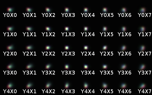
Fig.4 PSF sample points naming
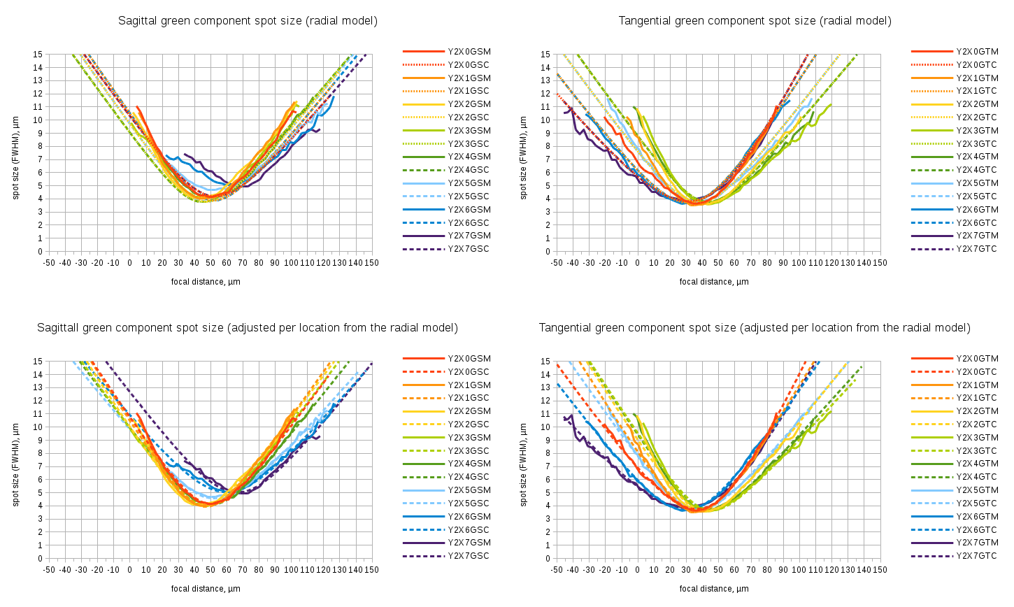
Fig.5 Fitting individual spot size functions to radial aberration model. Spreadsheet link
When I implemented the LMA and tried to find the best match (I was simultaneously adjusting the image plane tilt too) for the measured lens data, the residual difference was still large. Top two plots on Fig.5 show sagittal and tangential measured and modeled data for eight location along the center horizontal section of the image plane. Fig.4 explains the sample naming, linked spreadsheet contains full data for all sample locations and color/direction components. Solid lines show measured data, dashed – approximation by a radial model described above.
The residual fitting errors (especially for some lens samples) were significantly larger than if each sample location was fitted with individual parameters (the two bottom graphs on Fig.5). Even the best image plane tilt determined for sagittal and tangential components (if fitted separately) produced different results – one one lens the angle between the two planes reached 0.4°. The radial model graphs (especially for Y2X6 and Y2X7) show that the sagittal and tangential components are “pulling” the result in opposite directions It became obvious that the actual lenses can not be fully characterized in the terms of just the radial model as used for simulation of the designed lenses, the deviations of the symmetrical radial model have to be accounted for too.
Adjustment of the model parameters to accommodate per-location variations
I modified the initial fitting program to allow individual (per sample location) adjustment of the parameter values, adding cost of correction variation from zero and/or from the correction values of the same parameter at the neighbors sites. Sum of the squares of the corrections (with balanced weights) was added to the sum of the squares of the differences between the measured PSF sizes and the modeled ones. This procedure requires that small parameter variations result in small changes of the functions values, that was achieved by the modeling function formula modification as described above.
Lenses tested
New program was tested with 7 lens samples – 5 of them were used to evaluate individual variations of the same lens model, and the two others were different lenses. Each result image includes four graphs:
- Top-left graph shows weighted average resolution for each individual color and the combination of all three. Weighted average here processes the fourth power of the spot size at each of the 40 locations in both (sagittal and tangential) directions so the largest (worst) values have the highest influence on the result. This graph uses individually fitted spot size functions
- Bottom-left graph shows Petzval curvature for each of the 6 (2 directions of 3 colors) components. Dashed lines show sagittal and solid lines – tangential data for the radial model parameters, data point marks – the individually adjusted parameters, so same radius but different direction from the lens center results in the different values
- Top-right graph shows the resolution variation over radius for the plane at the “best” (providing highest composite resolution) distance from the lens, lines showing radial model data and marks – individual samples
- Bottom-right graph shows a family of the resolution functions for -10μm (closest to the lens), -5μm, 0μm, +50μm and +10μm positions of the image plane
Evetar N125B04518W
Evetar N125B04518W is our “workhorse” lens used in Eyesis cameras. 1/2.5″ format lens, focal length=4.5mm, F#=1.8. It is a popular product, and many distributors sell this lens under their own brand names. One of the reasons we are looking for the custom lens design is that while this lens has “W” in the model name suffix meaning “white” (as opposed to “IR” for infrared) it is designed to be a “one size fits all” product and the only difference is addition of the IR cutoff filter at the lens output. This causes two problems for our application – reduced performance for blue channel (and high longitudinal chromatic aberration for this color) and extra spherical aberration caused by the plane-parallel plate of the IR cutoff filter substrate. To mitigate the second problem we use non-standard very thin – just 0.3mm filters.
Below are the test results for 5 randomly selected samples of the batch of the lenses with different performance.
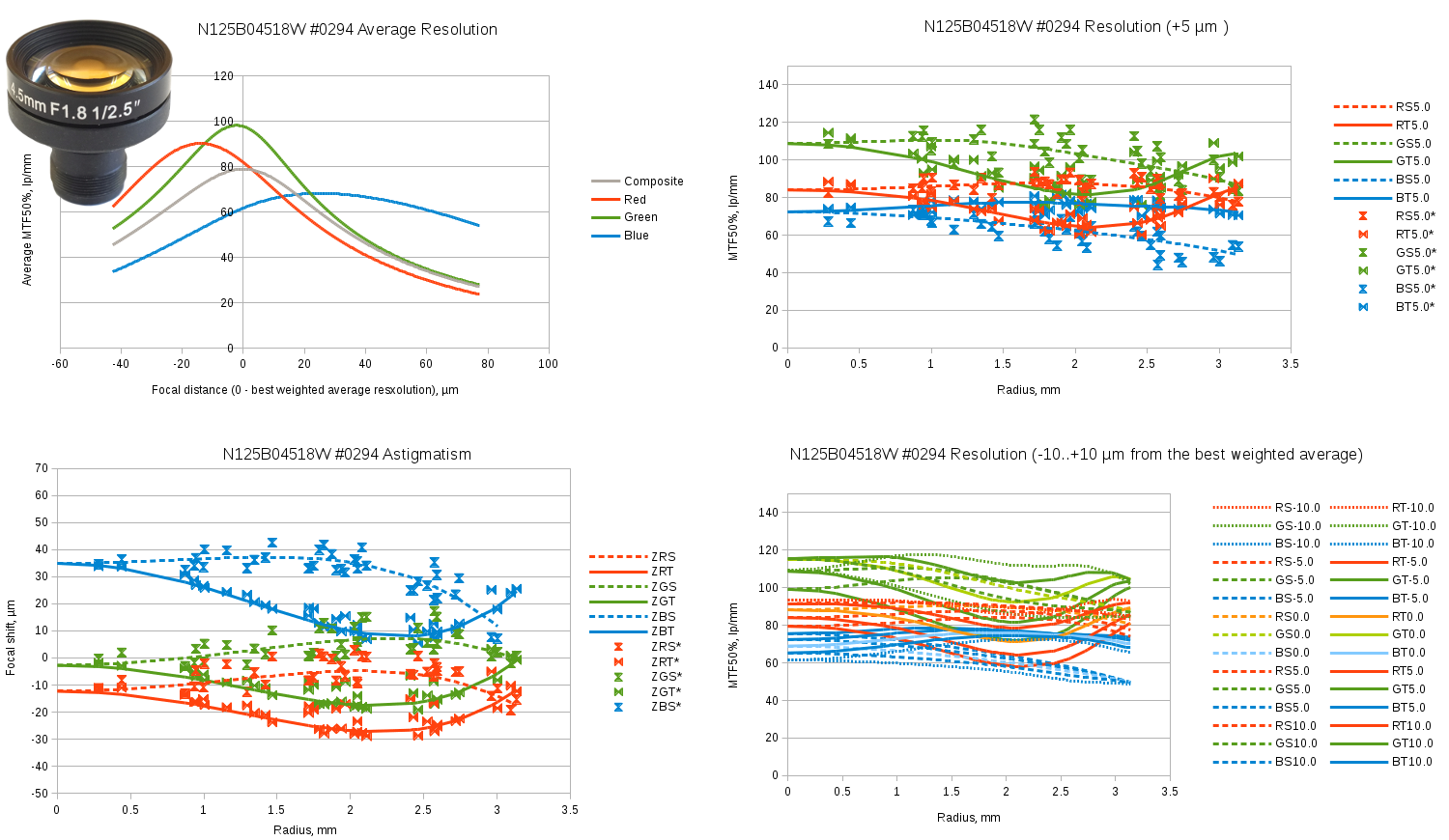
Fig.6 Evetar N125B04518W sample #0294 test results. Spreadsheet link.
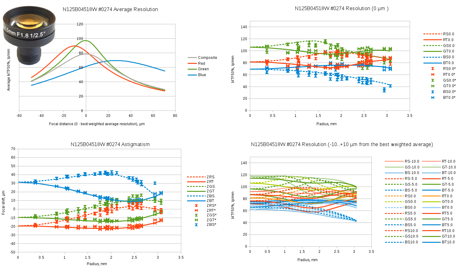
Fig.7 Evetar N125B04518W sample #0274 test results. Spreadsheet link.
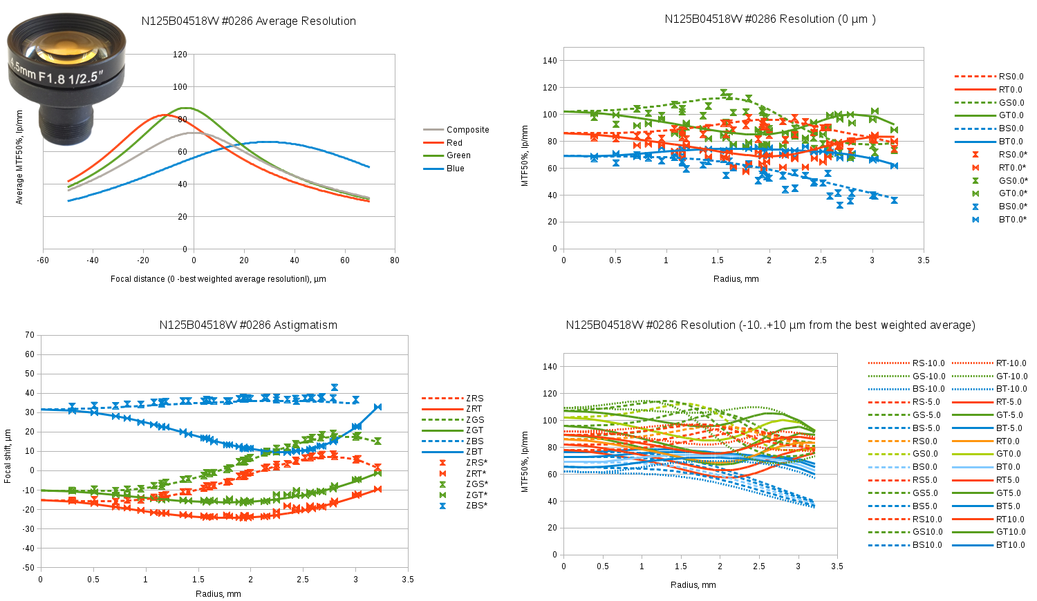
Fig.8 Evetar N125B04518W sample #0286 test results. Spreadsheet link.
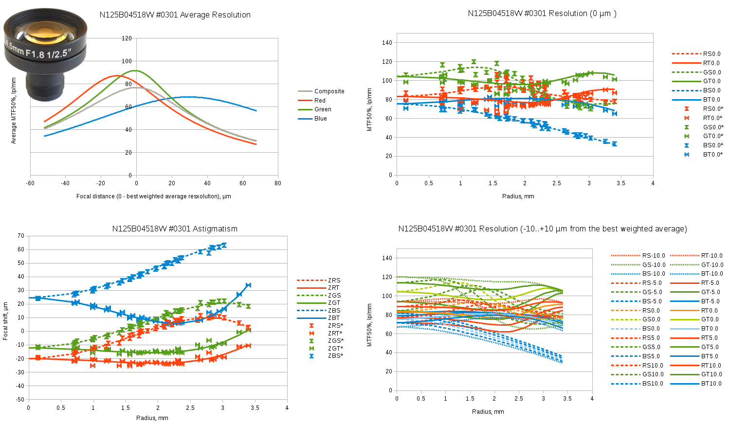
Fig.9 Evetar N125B04518W sample #0301 test results. Spreadsheet link.
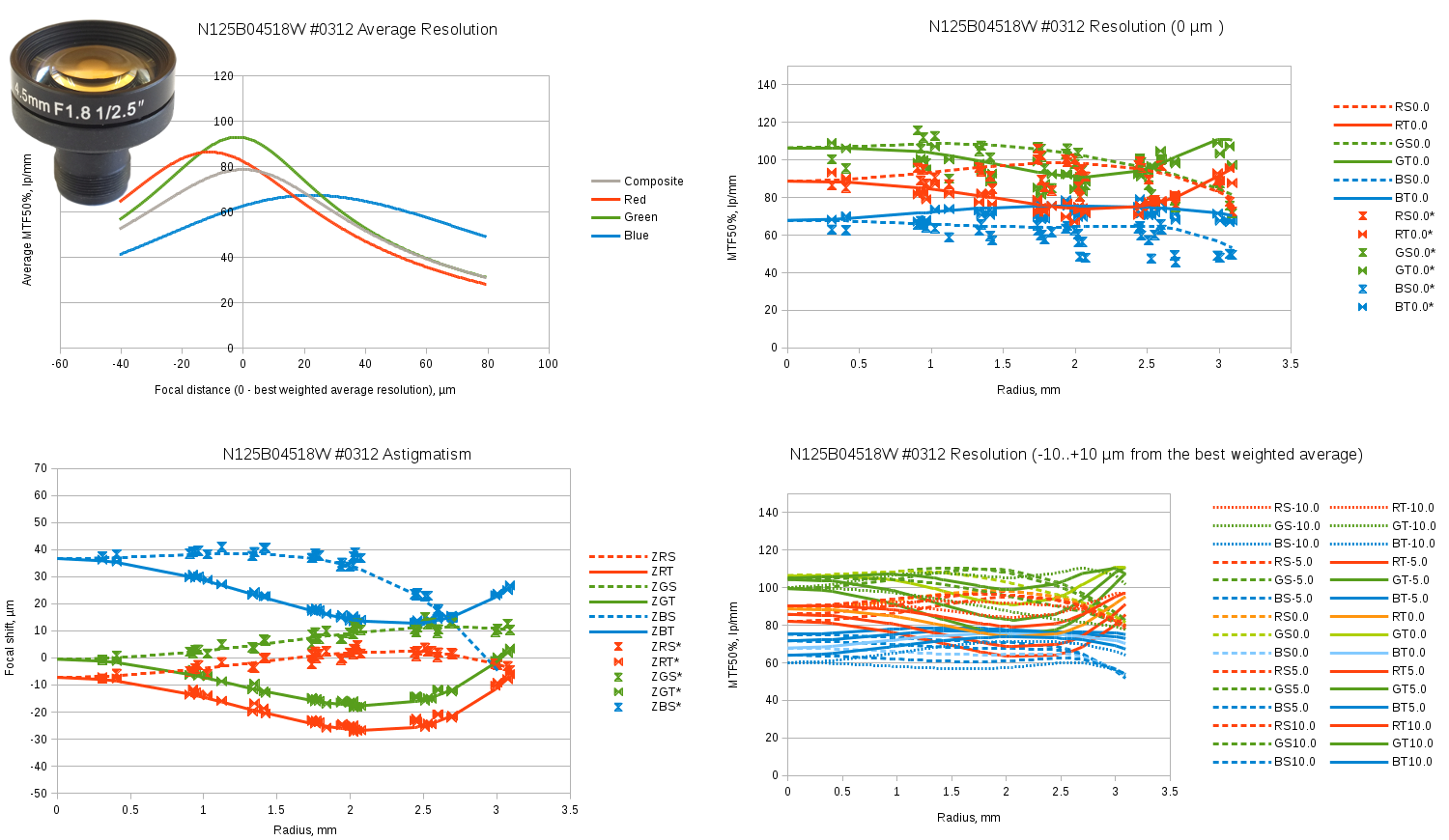
Fig.10Evetar N125B04518W sample #0312 test results. Spreadsheet link.
Evetar N125B04530W
High resolution 1/2.5″ f=4.5mm, F#=3.0 lens
Fig.11 Evetar N125B04530W sample #9101 test results. Spreadsheet link.
Sunex DSL945D
Sunex DSL945D – compact 1/2.3″ format f=5.5mm F#=2.5 lens. Datasheet says “designed for cameras using 10MP pixel imagers”. The sample we tested has very high center resolution, excellent image plane flatness and low chromatic aberrations. Unfortunately off-center resolution degrades with the radius rather fast.
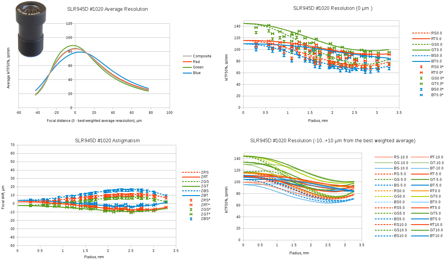
Fig.12 Sunex SLR945D sample #1020 test results. Spreadsheet link.
Sunex DSL355A-650-F2.8
Sunex DSL355A – 1/2.5″ format f=4.2mm F#=2.8 hybrid lens.
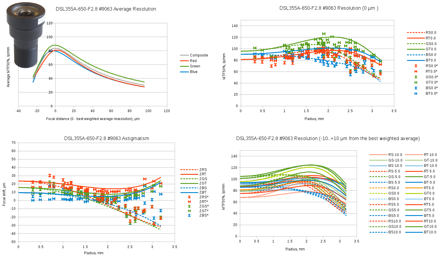
Fig.13 Sunex SLR355A sample #9063 test results. Spreadsheet link.
Software used
This project used Elphel plugin for the popular open source image processing program ImageJ with new classes implementing the new processing described here. The results were saved as text data tables and imported in free software LibreOffice Calc spreadsheet program to create visualization graphs. Finally free software Gimp program helped to combine graphs and create the animation of Fig.1.
Leave a Reply