Lens aberration correction with the lapped MDCT
Modern small-pixel image sensors exceed resolution of the lenses, so it is the optics of the camera, not the raw sensor “megapixels” that define how sharp are the images, especially in the off-center areas. Multi-sensor camera systems that depend on the tiled images do not have any center areas, so overall system resolution may be as low as that of is its worst part.
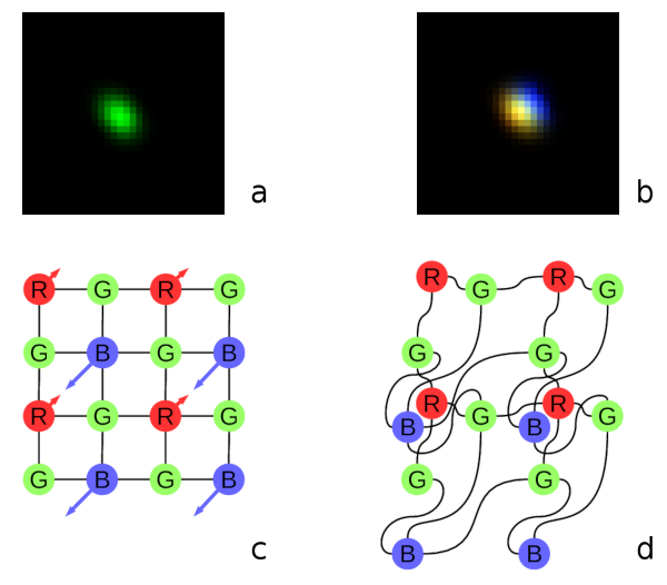
Fig. 1. Lateral chromatic aberration and Bayer mosaic: a) monochrome (green) PSF, b) composite color PSF, c) Bayer mosaic of the sensor, d) distorted mosaic for the chromatic aberration of b).
Contents
De-mosaic processing and chromatic aberrations
Our current cameras role is to preserve the raw sensor data while providing some moderate compression, all the image correction is applied during post-processing. Handling the lens aberration has to be done before color conversion (or de-mosaicing). When converting Bayer data to color images most cameras start with the calculation of the “missing” colors in the RG/GB pattern using 3×3 or 5×5 kernels, this procedure relies on the specific arrangement of the color filters.
Each of the red and blue pixels has 4 green ones at the same distance (pixel pitch) and 4 of the opposite (R for B and B for R) color at the equidistant diagonal locations. Fig.1. shows how lateral chromatic aberration disturbs these relations.
Fig.1a is the point-spread function (PSF) of the green channel of the sensor. The resolution of the PSF measurement is twice higher than the pixel pitch, so the lens is not that bad – horizontal distance between the 2 greens in Fig.1c corresponds to 4 pixels of Fig.1a. It is also clearly visible that the PSF is elongated and the radial resolution in this part of the image is better than the tangential one (lens center is left-down).
Fig.1b shows superposition of the 3 color channels: blue center is shifted up-and-right by approximately 2 PSF pixels (so one actual pixel period of the sensor) and the red one – half-pixel left-and-down from the green center. So the point light of a star, centered around some green pixel will not just spread uniformly to the two “R”s and two “B”s shown connected with lines in Fig.1c, but the other ones and in different order. Fig.1d illustrates the effective positions of the sensor pixels that match the lens aberration.
Aberrations correction at post-processing stage
When we perform off-line image correction we start with separating each color channel and re-sampling it at twice the pixel pitch frequency (adding zero sample between each measured one) – this increase allows to shift image by a fraction of a pixel both preserving resolution and not introducing the phase errors that may be visually OK but hurt when relying on sub-pixel resolution during correlation of images.
Next is the conversion of the full image into the overlapping square tiles to the frequency domain using 2-d DFT, then multiplication by the inverted PSF kernels – individual for each color channel and each part of the whole image (calibration procedure provides a 2-d array of PSF kernels). Such multiplication in the frequency domain is equivalent to (much more computationally expensive) image convolution (or deconvolution as the desired result is to reduce the effect of the convolution of the ideal image with the PSF of the actual lens). This is possible because of the famous convolution-multiplication property of Fourier transform and its discrete versions.
After each color channel tile is corrected and the phases of color components match (lateral chromatic aberration is compensated) it is the time when the data may be subject to non-linear processing that relies on the properties of the images (like detection of lines and edges) to combine the color channels trying to achieve highest spacial resolution and not to introduce color artifacts. Our current software performs it while data is in the frequency domain, before the inverse Fourier transform and merging the lapped tiles to the restored image.
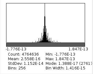
Fig.2. Histogram of difference between original image and after direct and inverse MDCT (with 8×8 pixels DCT-IV)
MDCT of an image – there and back again
It would be very appealing to use DCT-based MDCT instead of DFT for aberration correction. With just 8×8 point DCT-IV it may be possible to calculate direct 16×16 -> 8×8 MDCT and 8×8 -> 16×16 IMDCT providing perfect reconstruction of the image. 8×8 pixels DCT should be able to handle convolution kernels with 8 pixel radius – same would require 16×16 pixels DFT. I knew there will be a challenge to handle non-symmetrical kernels but first I gave a try to a 2-d MDCT to convert and reconstruct back a camera image that way. I was not able to find an efficient Java implementation of the DCT-IV so I had to write some code following the algorithms presented in [1].
That worked nicely – when I obtained a histogram of the difference between the original image (pixel values were in the range of 0 to 255) and the restored one – IMDCT(MDCT(original)) it demonstrated negligible error. Of course I had to discard 8 pixel border of the image added by replication before the procedure – these border pixels do not belong to 4 overlapping tiles as all internal ones and so can not be reconstructed.
When this will be done in the camera FPGA the error will be higher – DCT implementation there uses just an integer DSP – not capable of the double precision calculations as the Java code. But for the small 8×8 transformations it should be rather easy to manage calculation precision to the required level.
Convolution with MDCT
It was also easy to implement a low-pass symmetrical filter by multiplying 8×8 pixel MDCT output tiles by a DCT-III transform of the desired convolution kernel. To convolve f ☼ g you need to multiply DCT_IV(f) by DCT_III(g) in the transform domain [2], but that does not mean that DCT-III has also be implemented in the FPGA – the de-convolution kernels can be prepared during off-line calibration and provided to the camera in the required form.
But not much more can be done for the convolution with asymmetric kernels – they either require additional DST (so DCT and DST) of the image and/or padding data with extra zeros [3],[4] – all that reduces advantage of DCT compared to DFT. Asymmetric kernels are required for the lens aberration corrections and Fig.1 shows two cases not easily suitable for MDCT:
- lateral chromatic aberrations (or just shift in the image domain) – Fig.1b and
- “diagonal” kernels (Fig.1a) – not an even function of each of the vertical and horizontal axes.
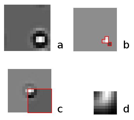
Fig.3. Convolution kernel factorization: a) required asymmetrical and shifted kernel, b) 4-point direct convolution with (sparse) Bayer color channel data, c) symmetric convolution kernel for MDCT, d) symmetric kernel – DCT-III of c) to multiply DCT-IV kernels of the image.
Symmetric kernels are like what you can do with a twice folded piece of paper, cut to some shape and unfolded, with folds oriented strictly vertically and horizontally.
Factorization of the convolution
Another way to handle convolution with non-symmetrical kernels is to split it in two – first convolve with an asymmetrical one directly and then – use MDCT and symmetrical kernel. The input data for combined convolution is split Bayer data, so each color channel receives sparse sequence – green one has only half non-zero elements and red and blue – only 1/4 such pixels. In the case of half-pixel grid (to handle fraction-pixel shifts) the relative amount of non-zero pixels is four times smaller, so the total number of multiplications is the same as for the whole-pixel grid.
The goal of such factorization is to minimize the number of the non-zero elements in the asymmetrical kernel, imposing no restrictions on the symmetrical one. Factorization does not have to be absolutely precise – the effect of deconvolution is limited by several factors, most important being the amplification of the sensor noise (such as shot noise). The required number of non-zero pixel may vary with the type of the distortion, for the lens we experimented with (Sunex DSL227 fisheye) just 4 pixels were sufficient to achieve 2-4% error for each of the kernel tiles. Four pixel kernels make it 1 multiplication per each of the red and blue pixels and 2 multiplications per green. As the kernels are calculated during the camera off-line calibration it should be possible to simultaneously generate scheduling of the the DSP and buffer memories to additionally reduce the required run-time FPGA resources.
Fig.3 illustrates how the deconvolution kernel for the aberration correction is split into two for the consecutive convolutions. Fig.1a shows the required deconvolution kernel determined during the existing calibration procedure. This kernel is shown far off-center even for the green channel – it appeared near the edge of the fish-eye lens field of view as the current lens model is based on the radial polynomial and is not efficient for the fish-eye (f-theta) lenses, so aberration correction by deconvolution had to absorb that extra shift. As the convolution kernel has fixed non-zero elements, the computation complexity does not depend on the maximal kernel dimensions. Fig.3b shows the determined asymmetric convolution kernel of 4 pixels, and Fig.3c – the kernel for symmetric convolution with MDCT, the unique 8×8 pixels part of it (inside of the red square) is replicated to the other3 quadrants by mirroring along row 0 and column 0 because of the whole pixel even symmetry – right boundary condition for DCT-III. Fig.3d contains result of the DCT-III applied to the data shown in Fig.3c.
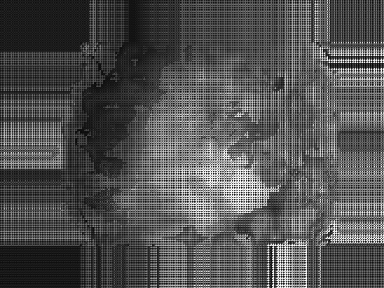
Fig.4. Symmetric convolution kernel tiles in MDCT domain. Full image (click to open) has peripheral kernels replicated as there was no calibration data outside of the fisheye lens filed of view
There should be some more efficient ways to find optimal combinations of the two kernels, currently I used a combination of the Levenberg-Marquardt Algorithm (LMA) that minimizes approximation error (root mean square of the differences between the given kernel and the result of the convolution of the two calculated) and adding/replacing pixels in the asymmetrical kernel, sorting the variants for the best LMA fit. Experimental code (FactorConvKernel.java) for the kernel calculation is in the same git repository.
Each kernel tile is processed independently of the neighbors, so while the aberration deconvolution kernels are changing smoothly between the adjacent tiles, the individual asymmetrical (for direct convolution with Bayer signal data) and symmetrical (for convolution by multiplication in the MDCT space) may change dramatically (see Fig.4). But when the direct convolution is applied before the window multiplication to the source pixels that contribute to a 16×16 pixel MDCT overlapping tile, then the result (after IMDCT) depends on the convolution of the two kernels, not the individual ones.
Deconvolving the test image
Next step was to apply the convolution to the test image, see if there are any visible blocking (or other) artifacts and if the image sharpness was improved. Only a single (green) channel was tested as there is no DCT-based color conversion code in this program yet. Program was tested with the whole pixel grid (not half pixel) so some reduction of sharpness caused by fractional pixel shift was expected. For the comparison “before/after” aberration correction I used two pairs – one with the raw Bayer data (half of the pixels are black in a checker-board pattern) and the other – with the Bayer pattern after 0.4 pix low-pass filter to reduce the checkerboard pattern. Without this filtering image would be either twice darker or (as on these pictures) saturated at lower levels (checkerboard 0/255 alternating pixels result in average gray level of only half of the full range).
Fig.5. Alternating images of a segment (green channel only): low-pass filter of the Bayer mosaic before and after deconvolution. Click image to show comparison with raw Bayer component.
Raw Bayer
Bayer data, low pass filter, sigma = 0.4 pix
Deconvolved
Fig.5 shows animated GIF of a fraction of the whole image, clicking the image shows comparison to the raw Bayer (with the limited gray level), caption links the full size images for these 3 modes.
No de-noise code is used, so amplification of the pixel shot noise is clearly visible, especially on the uniform surfaces, but aliasing cancellation remained functional even with abrupt changing of the convolution kernels as ones shown in Fig.4.
Conclusions
Algorithms suitable for FPGA implementation are tested with the simulation code. Processing of the images subject to the typical optical aberration of the fisheye lens DSL227 does not add significantly to the computational complexity compared to the pure symmetric convolution using lapped MDCT based on the 8×8 pixels two-dimensional DCT-IV.
This solution can be used as a first stage of the real time image correction and rectification, capable of sub-pixel resolution in multiple application areas, such as 3-d reconstruction and autonomous navigation.
References
[1] Plonka, Gerlind, and Manfred Tasche. “Fast and numerically stable algorithms for discrete cosine transforms.” Linear algebra and its applications 394 (2005): 309-345.
[2] Martucci, Stephen A. “Symmetric convolution and the discrete sine and cosine transforms.” IEEE Transactions on Signal Processing 42.5 (1994): 1038-1051. pdf
[3] Suresh, K., and T. V. Sreenivas. “Linear filtering in DCT IV/DST IV and MDCT/MDST domain.” Signal Processing 89.6 (2009): 1081-1089. Abstract and full text pdf.
[4] Reju, Vaninirappuputhenpurayil Gopalan, Soo Ngee Koh, and Ing Yann Soon. “Convolution using discrete sine and cosine transforms.” IEEE Signal Processing Letters 14.7 (2007): 445. pdf
[5] Malvar, Henrique S. “Extended lapped transforms: Properties, applications, and fast algorithms.” IEEE Transactions on Signal Processing 40.11 (1992): 2703-2714.
Leave a Reply