Lapped MDCT-based image conditioning with optical aberrations correction, color conversion, edge emphasis and noise reduction
Contents
Results of the processing of the color image
Previous blog post “Lens aberration correction with the lapped MDCT” described our experiments with the lapped MDCT[1] for optical aberration corrections of a single color channel and separation of the asymmetrical kernel into a small asymmetrical part for direct convolution and a larger symmetrical one to be applied in the frequency domain of the MDCT. We supplemented this processing chain with additional steps of the image conditioning to evaluate the overall quality of the of the results and feasibility of the MDCT approach for processing in the camera FPGA.
Image comparator in Fig.1 allows to see the difference between the images generated from the results of the several stages of the processing. It makes possible to compare any two of the image layers by either sliding the image separator or by just clicking on the image – that alternates right/left images. Zoom is controlled by the scroll wheel (click on the zoom indicator fits image), pan – by dragging.
Original image was acquired with Elphel model 393 camera with 5 Mpix MT9P006 image sensor and Sunex DSL227 fisheye lens, saved in jp4 format as a raw Bayer data at 98% compression quality. Calibration was performed with the Java program using calibration pattern visible in the image itself. The program is designed to work with the low-distortion lenses so fisheye was a stretch and the calibration kernels near the edges are just replicated from the ones closer to the center, so aberration correction is only partial in those areas.
First two layers differ just by added annotations, they both show output of a simple bilinear demosaic processing, same as generated by the camera when running in JPEG mode. Next layers show different stages of the processing, details are provided later in this blog post.
Linear part of the image conditioning: convolution and color conversion
Correction of the optical aberrations in the image can be viewed as convolution of the raw image array with the space-variant kernels derived from the optical point spread functions (PSF). In the general case of the true space-variant kernels (different for each pixel) it is not possible to use DFT-based convolution, but when the kernels change slowly and the image tiles can be considered isoplanatic (areas where PSF remains the same to the specified precision) it is possible to apply the same kernel to the whole image tile that is processed with DFT (or combined convolution/MDCT in our case). Such approach is studied in deep for astronomy [2],[3] (where they almost always have plenty of δ-function light sources to measure PSF in the field of view :-)).
The procedure described below is a combination of the sparse kernel convolution in the space domain with the lapped MDCT processing making use of its perfect (only approximate with the variant kernels) reconstruction property, but it still implements the same convolution with the variant kernels.
Signal flow is presented in Fig.2. Input signal is the raw image data from the sensor sampled through the color filter array organized as a standard Bayer mosaic: each 2×2 pixel tile includes one of the red and blue samples, and 2 of the green ones.
In addition to the image data the process depends on the calibration data – pairs of asymmetrical and symmetrical kernels calculated during camera calibration as described in the previous blog post.
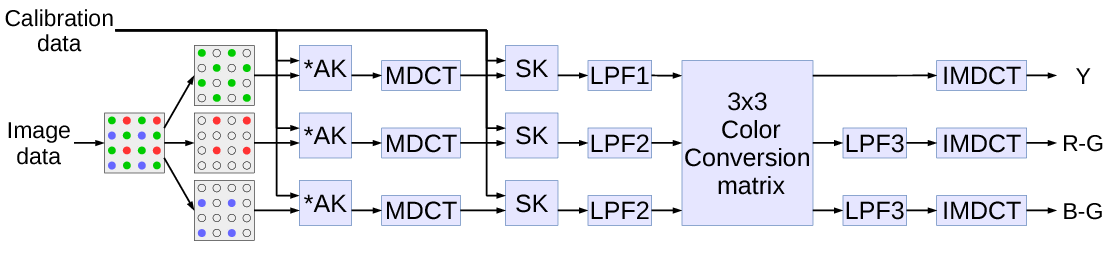
Fig.2. Signal flow of the linear part of MDCT-based image conditioning
Image data is processed in the following sequence of the linear operations, resulting in intensity (Y) and two color difference components:
- Input composite signal is split by colors into 3 separate channels producing sparse data in each.
- Each channel data is directly convolved with a small (we used just four non-zero elements) asymmetrical kernel AK, resulting in a sequence of 16×16 pixel tiles, overlapping by 8 pixels (input pixels are not limited to 16×16 tiles).
- Each tile is multiplied by a window function, folded and converted with 8×8 pixel DCT-IV[4] – equivalent of the 16×16->8×8 MDCT.
- 8×8 result tiles are multiplied by symmetrical kernels (SK) – equivalent of convolving the pre-MDCT signal.
- Each channel is subject to the low-pass filter that is implemented by multiplying in the frequency domain as these filters are indeed symmetrical. The cutoff frequency is different for the green (LPF1) and other (LPF2) colors as there are more source samples for the first. That was the last step before inverse transformation presented in the previous blog post, now we continued with a few more.
- Natural images have strong correlation between different color channels so most image processing (and compression) algorithms involve converting the pure color channels into intensity (Y) and two color difference signals that have lower bandwidth than intensity. There are different standards for the color conversion coefficients and here we are free to use any as this process is not a part of a matched encoder/decoder pair. All such conversions can be represented as a 3×3 matrix multiplication by the (r,g,b) vector.
- Two of the output signals – color differences are subject to an additional bandwidth limiting by LPF3.
- IMDCT includes 8×8 DCT-IV, unfolding 8×8 into 16×16 tiles, second multiplication by the window function and accumulation of the overlapping tiles in the pixel domain.
Nonlinear image enhancement: edge emphasis, noise reduction
For some applications the output data is already useful – ideally it has all the optical aberrations compensated so the remaining far-reaching inter-pixel correlation caused by a camera system is removed. Next steps (such as stereo matching) can be done on- (or off-) line, and the algorithms do not have to deal with the lens specifics. Other applications may benefit from additional processing that improves image quality – at least the perceived one.
Such processing may target the following goals:
- To reduce remaining signal modulation caused by the Bayer pattern (each source pixel carries data about a single color component, not all 3), trying to remove it by a LPF would blur the image itself.
- Detect and enhance edges, as most useful high-frequency elements represent locally linear features
- Reduce visible noise in the uniform areas (such as blue sky) where significant (especially for the small-pixel sensors) noise originates from the shot noise of the pixels. This noise is amplified by the aberration correction that effectively increases the high frequency gain of the system.
Some of these three goals overlap and can be addressed simultaneously – edge detection can improve de-mosaic quality and reduce related colored artifacts on the sharp edges if the signal is blurred along the edges and simultaneously sharpened in the orthogonal direction. Areas that do not have pronounced linear features are likely to be uniform and so can be low-pass filtered.
The non-linear processing produces modified pixel value using 3×3 pixel array centered around the current pixel. This is a two-step process:
- First the 3×3 center-symmetric matrices (one for Y, another for color) of coefficients are calculated using the Y channel data, then
- they are applied to the Y and color components by replacing the pixel value with the inner product of the calculated coefficients and the original data.
Signal flow for one channel is presented in Fig.3:
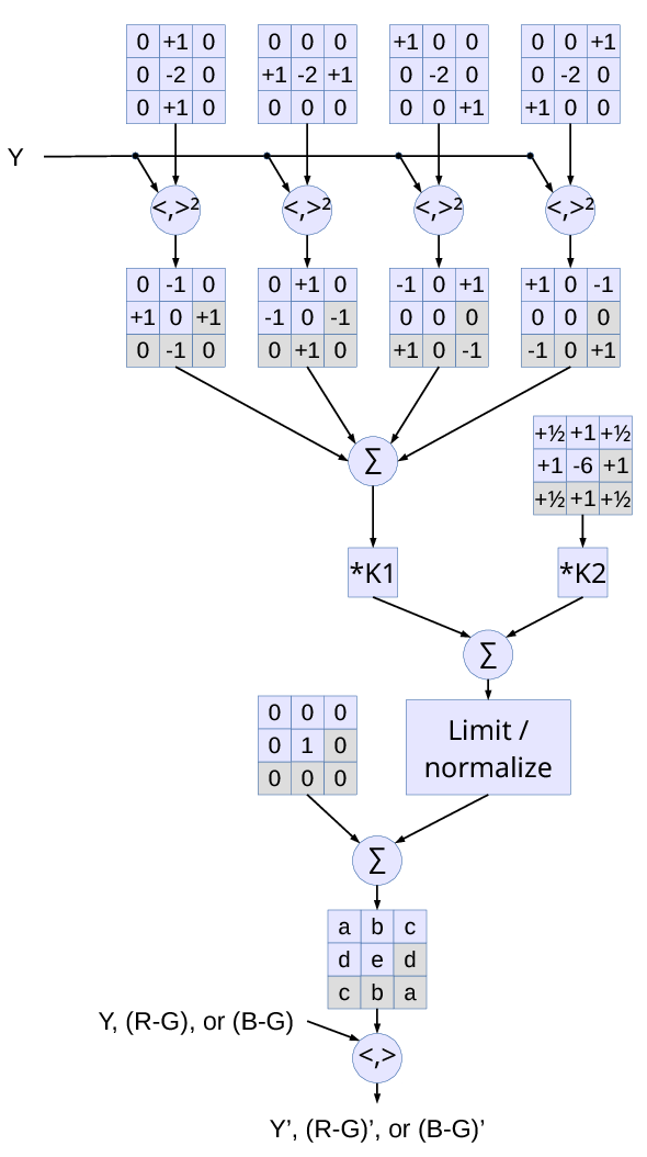
Fig.3 Non-linear image processing: edge emphasis and noise reduction
- Four inner products are calculated for the same 9-sample Y data and the shown matrices (corresponding to second derivatives along vertical, horizontal and the two diagonal directions).
- Each of these values is squared and
- the following four 3×3 matrices are multiplied by these values. Matrices are symmetrical around the center, so gray-colored cells do not need to be calculated.
- Four matrices are then added together and scaled by a variable parameter K1. The first two matrices are opposite to each other, and so are the second two. So if the absolute value of the two orthogonal second derivatives are equal (no linear features detected), the corresponding matrices will annihilate each other.
- A separate 3×3 matrix representing a weighted running average, scaled by K2 is added for noise reduction.
- The sum of the positive values is compared to a specified threshold value, and if it exceed it – all the matrix is proportionally scaled down – that makes different line directions to “compete” against each other and against the blurring kernel.
- The sum of all 9 elements of the calculated array is zero, so the default unity kernel is added and when correction coefficients are zeros, the result pixels will be the same as the input ones.
- Inner product of the calculated 9-element array and the input data is calculated and used as a new pixel value. Two of the arrays are created from the same Y channel data – one for Y and the other for two color differences, configurable parameters (K1, K2, threshold and the smoothing matrix) are independent in these two cases.
Next steps
How much is it possible to warp?
The described method of the optical aberration correction is tested with the software implementation that uses only operations that can be ported to the FPGA, so we are almost ready to get back to to Verilog programming. One more thing to try before is to see if it is possible to merge this correction with a minor distortion correction. DFT and DCT transforms are not good at scaling the images (when using the same pixel grid). It is definitely not possible no rectify large areas of the fisheye images, but maybe small (fraction of a pixel per tile) stretching can still be absorbed in the same step with shifting? This may have several implications.
Single-step image rectification
It would be definitely attractive to eliminate additional processing step and save FPGA resources and/or decrease the processing time. But there is more than that – re-sampling degrades image resolution. For that reason we use half-pixel grid for the offline processing, but it increases amount of data 4 times and processing resources – at least 4 times also.
When working with the whole pixel grid (as we plan to implement in the camera FPGA) we already deal with the partial pixel shifts during convolution for aberration correction, so it would be very attractive to combine these two fractional pixel shifts into one (calibration process uses half-pixel grid) and so to avoid double re-sampling and related image degrading.
Using analytical lens distortion model with the precision of the pixel mapping
Another goal that seems achievable is to absorb at least the table-based pixel mapping. Real lenses can only to some precision be described by an analytical formula of a radial distortion model. Each element can have errors and the multi-lens assembly can inevitably has some mis-alignments – all that makes the lenses different and deviate from a perfect symmetry of the radial model. When we were working with (rather low distortion) wide angle lenses Evetar N125B04530W we were able to get to 0.2-0.3 pix root mean square of the reprojection error in a 26-lens camera system when using radial distortion model with up to the 8-th power of the radial polynomial (insignificant improvement when going from 6-th to the 8-th power). That error was reduced to 0.05..0.07 pixels when we implemented table-based pixel mapping for the remaining (after radial model) distortions. The difference between one of the standard lens models – polynomial for the low-distortion ones and f-theta for fisheye and “f-theta” lenses (where angle from optical axis approximately linearly depends on the distance from the center in the focal plane) is rather small, so it is a good candidate to be absorbed by the convolution step. While this will not eliminate re-sampling when the image will be rectified, this distortion correction process will have a simple analytical formula (already supported by many programs) and will not require a full pixel mapping table.
High resolution Z-axis (distance) measurement with stereo matching of multiple images
Image rectification is an important precondition to perform correlation-based stereo matching of two or more images. When finding the correlation between the images of a relatively large and detailed object it is easy to get resolution of a small fraction of a pixel. And this proportionally increases the distance measurement precision for the same base (distance between the individual cameras). Among other things (such as mechanical and thermal stability of the system) this requires precise measurement of the sub-camera distortions over the overlapping field of view.
When correlating multiple images the far objects (most challenging to get precise distance information) have low disparity values (may be just few pixels), so instead of the complete rectification of the individual images it may be sufficient to have a good “mutual rectification”, so the processed images of the object at infinity will match on each of the individual images with the same sub-pixel resolution as we achieved for off-line processing. This will require to mechanically orient each sub-camera sensor parallel to the others, point them in the same direction and preselect lenses for matching focal length. After that (when the mechanical match is in reasonable few percent range) – perform calibration and calculate the convolution kernels that will accommodate the remaining distortion variations of the sub-cameras. In this case application of the described correction procedure in the camera will result in the precisely matched images ready for correlation.
These images will not be perfectly rectified, and measured disparity (in pixels) as well as the two (vertical and horizontal) angles to the object will require additional correction. But this X/Y resolution is much less critical than the resolution required for the Z-measurements and can easily tolerate some re-sampling errors. For example, if a car at a distance of 20 meters is viewed by a stereo camera with 100 mm base, then the same pixel error that corresponds to a (practically negligible) 10 mm horizontal shift will lead to a 2 meter error (10%) in the distance measurement.
References
[1] Malvar, Henrique S. Signal processing with lapped transforms. Artech House, 1992.
[2] Thiébaut, Éric, et al. “Spatially variant PSF modeling and image deblurring.” SPIE Astronomical Telescopes+ Instrumentation. International Society for Optics and Photonics, 2016. pdf
[3] Řeřábek, M., and P. Pata. “The space variant PSF for deconvolution of wide-field astronomical images.” SPIE Astronomical Telescopes+ Instrumentation. International Society for Optics and Photonics, 2008.pdf
[4] Britanak, Vladimir, Patrick C. Yip, and Kamisetty Ramamohan Rao. Discrete cosine and sine transforms: general properties, fast algorithms and integer approximations. Academic Press, 2010.
Leave a Reply