Efficient Complex Lapped Transform Implementation for the Space-Variant Frequency Domain Calculations of the Bayer Mosaic Color Images
This post continues discussion of the small tile space-variant frequency domain (FD) image processing in the camera, it demonstrates that modulated complex lapped transform (MCLT) of the Bayer mosaic color images requires almost 3 times less computational resources than that of the full RGB color data.
Contents
“Small Tile” and “Space Variant”
Why “small tile“? Most camera images have short (up to few pixels) correlation/mutual information span related to the acquisition system properties – optical aberrations cause a single scene object point influence a small area of the sensor pixels. When matching multiple images increase of the window size reduces the lateral (x,y) resolution, so many of the 3d reconstruction algorithms do not use any windows at all, and process every pixel individually. Other limitation on the window size comes from the fact that FD conversions (Fourier and similar) in Cartesian coordinates are shift-invariant, but are sensitive to scale and rotation mismatch. So targeting say 0.1 pixel disparity accuracy the scale mismatch should not cause error accumulation over window width exceeding that value. With 8×8 tiles (16×16 overlapped) acceptable scale mismatch (such as focal length variations) should be under 1%. That tolerance is reasonable, but it can not get much tighter.
What is “space variant“? One of the most universal operations performed in the FD is convolution (also related to correlation) that exploits convolution-multiplication property. Mathematically convolution applies the same operation to each of the points of the source data, so shifted object of the source image produces just a shifted result after convolution. In the physical world it is a close approximation, but not an exact one. Stars imaged by a telescope may have sharper images in the center, but more blurred in the peripheral areas. While close (angularly) stars produce almost the same shape images, the far ones do not. This does not invalidate convolution approach completely, but requires kernel to (smoothly) vary over the input images [1, 2], makes it a space-variant kernel.
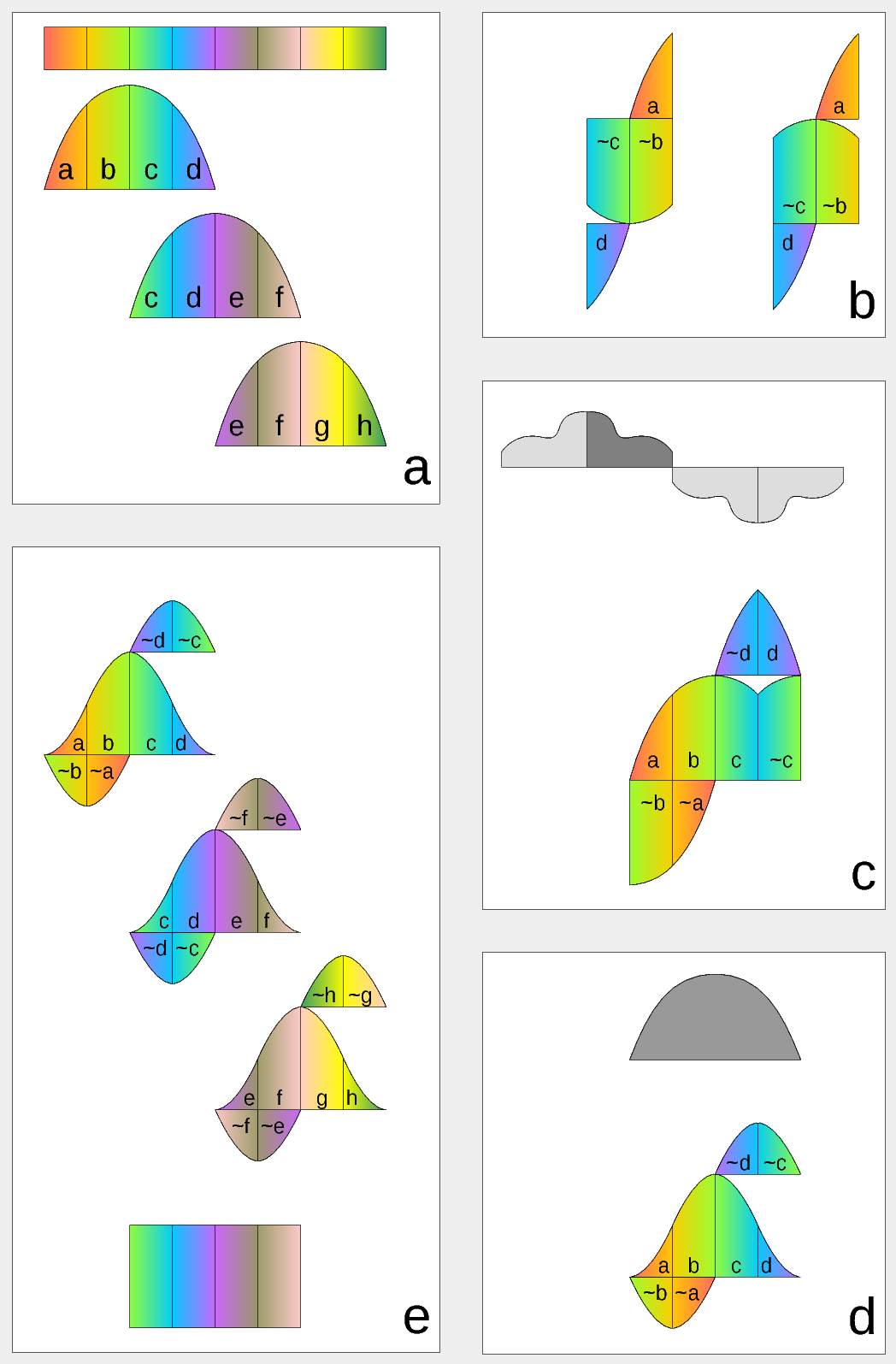
Figure 1. Complex Lapped Transform with DCT-IV/DST-IV: time-domain aliasing cancellation (TDAC) property. a) selection of overlapping input subsequences 2*N-long, multiplication by sine window; b) creating N-long sequences for DCT-IV (left) and DST-IV (right); c) (after frequency domain processing) extending N-long sequence using DCT-IV boundary conditions (DST-IV processing is similar); d) second multiplication by sine window; e) combining partial data
There is another issue related to the space-variant kernels. Fractional pixel shifts are required for multiple steps of the processing: aberration correction (obvious in the case of the lateral chromatic aberration), image rectification before matching that accounts for lens optical distortion, camera orientation mismatch and epipolar geometry transformations. Traditionally it is handled by the image rectification that involves re-sampling of the pixel values for a new grid using some type of the interpolation. This process distorts the signal data and introduces non-linear errors that reduce accuracy of the correlation, that is important for subpixel disparity measurements. Our approach completely eliminates resampling and combines integer pixel shift in the pixel domain and delegates the residual fractional pixel shift (±0.5 pix) to the FD, where it is implemented as a cosine/sine phase rotator. Multiple sources of the required pixel shift are combined for each tile, and then a single phase rotation is performed as a last step of pixel domain to FD conversion.
Frequency Domain Conversion with the Modulated Complex Lapped Transform
Modulated Complex Lapped Transform (MCLT)[3] can be used to split input sequence into overlapping fractions, processed separately and then recombined without block artifacts. Popular application is the signal compression where “processed separately” means compressed by the encoder (may be lossy) and then reconstructed by the decoder. MCLT is similar to the MDCT that is implemented with DCT-IV, but it additionally preserves and allows frequency domain modification of the signal phase. This feature is required for our application (fractional pixel shifts and asymmetrical lens aberrations modify phase), and MCLT includes both MDCT and MDST (that use DCT-IV and DST-IV respectively). For the image processing (2d conversion) four sub-transforms are needed:
- horizontal DCT-IV followed by vertical DCT-IV
- horizontal DST-IV followed by vertical DCT-IV
- horizontal DCT-IV followed by vertical DST-IV
- horizontal DST-IV followed by vertical DST-IV
Reversibility of the Modified Discrete Cosine and Sine Transforms
Figure 1 illustrates the principle of TDAC (time-domain aliasing cancellation) that restores initial data from the series of individually converted subsections after seemingly lossy transformations. Step a) shows the 2*N long (in our case N=8) data subsets extraction, each subset is multiplied by a window function. It is a half period of the sine function, but other windows are possible as long as they satisfy the Princen-Bradley condition. Each of the sections corresponds to N/2 of the input samples, color gradients indicate input order. Figure 2b has seemingly lossy result of MDCT (left) and MDST (right) performed on the 2*N long input resulting in N-long – tilde indicates time-reversal of the subsequence (image has the gradient direction reversed too). Upside-down pieces indicate subtraction, up-right – addition. Each of the 2*N → N transforms is irreversible by itself, TDAC depends on the neighbor sections.
Figure 1c shows the first step of original sequence restoration, it extends N-long sequence using DCT-IV boundary conditions – it continues symmetrically around left boundary, and anti-symmetrically around the right one (both around half-sample from the first/last one), behaving like a first quadrant (0 to π/2) of the cosine function. Conversions for DST branch are not shown, they are similar, just extended like a first quadrant of the sine function.
The result sequence of step c) (now 2*N long again) is multiplied by the window function for the second time in step d), the two added terms of the last column ( and ) are swapped for clarity.
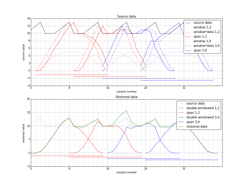
Figure 2. Space-variant phase shift (extra overlap), source-centered window. Distorted reconstruction in the center
The last image e) places result of the step d) and those of similarly processed subsequences and to the same time line. Fraction of the first block compensates of the second, and of the second – of the third. As the window satisfies Princen-Bradley condition, and it is applied twice, the columns of the first and second block when added result in segment of the original sequence. The same is true for the , , and columns. First and last N samples are not restored as there are no respective left and right neighbors to be processed.
Space-variant shift and TDAC property
Modified discrete cosine and sine transforms exhibit a perfect reconstruction property when input sequence is split into regular overlapping intervals and this is the case for many applications, such as audio and video compression. But what happens in the case of a space-variant shift? As the total shift is split into integer and symmetrical fractional part even smooth variation of the required shift for the neighbor sample sequences there will be places where the required shift crosses ±0.5 pix boundaries. This will cause the overlap to be N±1 instead of exactly N and the remaining fractional pixel shift will jump from +0.5 pix to -0.5pix or vice versa.
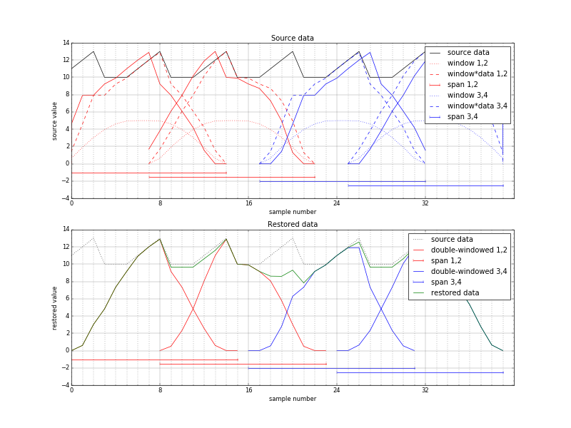
Figure 3. Space-variant phase shift (reduced overlap), source-centered window. Distorted reconstruction in the center
Such condition is illustrated in Figure 2, where fractional pixel shift is increased to ±1.0 instead of ±0.5 to avoid signal shape distortion caused by a fractional shift. The sine window is also modified accordingly to have zeros on both ends and so to have a flat top, but it still satisfies Princen-Bradley condition. The sawtooth waveform represents input signal that has large pedestal = 10 and a full amplitude of 3. The two left input intervals (1 to 16 and 9 to 24) are shown in red, the two right ones (15 to 30 and 23 to 38) are blue. These intervals have extra overlap (N+2) between red and blue ones. Dotted waveforms show window functions centered around input intervals, dashed – inputs multiplied by the windows. Solid lines on the top plot show result of the FD rotation resulting in 1 shift to the right for the red subsequences, to the left – by the blue ones.
The bottom plot of Figure 2 is for the “rectified image”, where the overlapping intervals are spread evenly (0-15, 8-23, 16-31, 24-39), the restored data is multiplied by the windows again (red and blue solid lines) and then added together (dark green waveform) in an attempt to restore the original sawtooth.
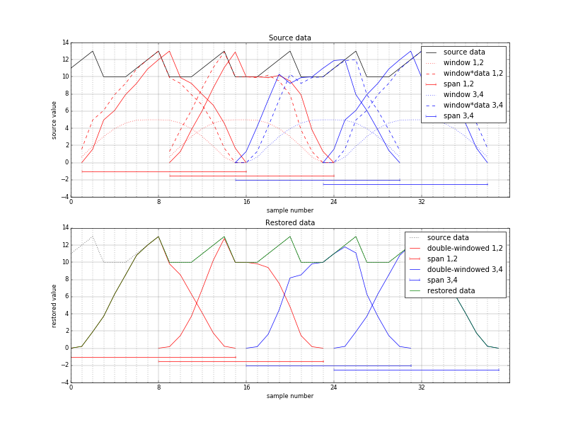
Figure 4. Space-variant phase shift (extra overlap), modified window. Correct reconstruction
There is an obvious problem in the center where the peak is twice higher than the center sawtooth (dotted waveform). It is actually a “wrinkle” caused by the input signal pedestal that was pushed to the center by the increased overlap of the input, not by the sawtooth shape. The FD phase shift moved windowed input signal, not just the input signal. So even if the input signal was constant, left two windows would be shifted right by 1, and right ones – left by one sample, distorting their sum. Figure 3 illustrates the opposite case where the input subsequences have reduced rather than increased overlap and FD phase rotation moves windowed data away from the center – the restored signal has a dip in the middle.
This problem can be corrected if the first window function used for input signal multiplication takes the FD shift into account, so that the input windows after phase rotation match the output ones. Signals similar to those in Figure 2, but with appropriately offset input windows (dotted waveforms are by 1 pixel asymmetrical) are presented in Figure 4. It shows perfect reconstruction (dark green line) of the offset input sawtooth signal.
Implementation of the MCLT for the Monochrome 16×16 Pixel Tiles

Figure 5. MCLT converter for the 16×16 pixel tiles
The MCLT converter illustrated in Figure 5 takes an array of 256 pixel samples and processes them at the rate of 1 pixel per clock, resulting in 4 of the 64 (8×8) arrays representing FD transformation of this tile. Converter incorporates phase rotator that is equivalent to the fractional pixel shifter with 1/128 pixel resolution. Multiple pixel tiles tiles can be processed immediately after each other or with a minimal gap of 16 pixels needed to restore the pipeline state. Fold sequencer receives start signal and simultaneously two 7-bit fractional pixel X and Y shifts in 1/128 increments (-64 to +63). Pixel data is received from the read-only port of the dual-port memory (input tile buffer) filled from the external DDR memory. Fold sequencer generates buffer addresses (including memory page number) and can be configured for various buffer latency.

Figure 6. DCT-IV and DST-IV basis functions for N=8
Fold sequencer simultaneously generates X and Y addresses for the 2-port window ROM that generates window function (it is a half-sine as discussed above) values that are combined by a multiplier as the 2-d window function is separable. Each of the dimensions calculate window values with appropriate subpixel shift to allow space-variant FD processing. Mapping from the 16×16 to 8×8 tiles is performed according to Figure 1b for each direction, resulting in four 8×8 tiles for DCT/DCT (horizontal/vertical), DST/DCT, DCT/DST and DST/DST future processing, Each of the source pixels contribute to all 4 of the 8×8 arrays, and each corresponding elements of the 4 output arrays share the same 4 contributing pixels – just with different signs. That allows to iterate through the source pixels in groups of 4 once, multiply them by appropriate window values and in 4 cycles add/subtract them in 4 accumulators. These values are registered and multiplexed during the next 4 cycles feeding 512×25 DTT input buffer (DTT stands for Discrete Trigonometric Transform – a collective name for both DCT and DST).
“Folded” data stored in the 512×25 DTT input buffer is fed to the 2-dimensional 8×8 pixel DTT module. It is similar to the one described in the DCT-IV implementation blog post, it was just modified to allow all 4 DTT variants, not just the DCT/DCT described there. This was done using the property of DCT-IV/DST-IV that DST-IV can be calculated as DCT-IV if the input sequence is reversed (x0 ↔ x7, x1 ↔ x6, x2 ↔ x5, x3 ↔ x4) and sign of the odd output samples (y1, y3, y5, y7) is inverted. This property can be seen by comparing plots of the basis functions in Figure 6, the proof will be later in the text.

Figure 7. Frequency domain phase rotator
Another memory buffer is needed after the 2d DTT module as it processes one of four 64-pixel transforms at a time, and the phase rotator (Figure 7) needs simultaneous access to all 4 components of the same FD sample. These 4 components are shown on the left of the diagram, they are multiplied by 4 sine/cosine values (shown as CH, SH, CV and SV) and then combined by the adders/subtracters. Total number of multiplications is 16, and they have to be performed it 4 clock cycles to maintain the same data rate through all the MCLT converter, so 4 multiplier-accumulator modules are needed. One FD point calculation uses 4 different sine/cosine coefficients, so a single ROM is sufficient. The phase rotator uses horizontal and vertical fractional pixel shift values for the second time (first was for the window function) and combines them with the multiplexed horizontal and vertical indexes (3 bits each) as address inputs of the coefficient ROM. Rotator provides rotated coefficients that correspond to the MCLT transform of the pixel data shifted in both horizontal and vertical directions by up to ±0.5 pix at a rate of 1 coefficient per clock cycle, providing both output data and address to the external multi-page memory buffer.
Modulated Complex Lapped Transform for the Bayer Mosaic Color Images
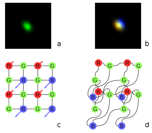
Fig. 8. Lateral chromatic aberration and the Bayer mosaic: a) monochrome (green) PSF, b) composite color PSF, c) Bayer mosaic of the sensor (direction of aberration shown), d) distorted mosaic matching chromatic aberration of b).
Most camera applications use color image sensors that provide Bayer mosaic color data: one red, one blue and two diagonal green pixels in each 2×2 pixel group. In old times image senor pixel density was below the lenses optical resolution and all the cameras performed color interpolation (usually bilinear) of the “missing” colors. This process implied that each red pixel, for example, had four green neighbors (up, down, left and right) at equal distance, and 4 blue pixels located diagonally. With the modern high-resolution sensors it is not the case, possible distortions are shown on Figure 8 (copied from the earlier post). More elaborate “de-mosaic” processing involves non-linear operations that would influence sub-pixel correlation results.
As the simple de-mosaic procedures can not be applied to the high resolution sensors without degrading the images, we treat each color subchannel individually, merging results after performing the optical aberration correction in the FD, or at least compensating the lateral chromatic aberration that causes pixels x/y shift.
Channel separation means that when converting data to the FD the input data arrays are decimated: for green color only half of the values (located in a checkerboard pattern) are non-zero, and for red and blue subchannels – only quarter of all pixels have non-zero values. The relative phase of the remaining pixels depends on the required integer pixel offset (only ±0.5 are delegated to the FD) and may have 2 values (black vs. white checkerboard cells) for green, and 4 different values (odd/even for each of the horizontal/vertical directions independently) for red and blue. MCLT can be performed on the sparse input arrays the same way as on the complete 16×16 ones, low-pass filters (LPF) may be applied on the later processing stages (LPF may be applied to the deconvolution kernels used for aberration correction during camera calibration). It is convenient to multiply red and blue values by 2 to compensate for the smaller number of participating pixels compared to the green sub-channel.
Direct approach to calculate FD transformation of the color mosaic input image would be to either run the monochrome converter (Figure 5) three times (in 256*3=768 clock cycles) masking out different pixel pattern each time, or implement the same module (including the input pixel buffer) three times to achieve 256 clock cycle operation. And actually the 16×16 pixel buffer used in monochrome converter is not sufficient – even the small lateral chromatic aberration leads to mismatch of the 16×16 tiles for different colors. That would require using larger – 18×18 (for minimal aberration) pixel buffer or larger if that aberration may exceed a full pixel.
Luckily MCLT that consists of MDCT and MDST, they it turn use DCT-IV and DST-IV that have a very convenient property when processing the Bayer mosaic data. Almost the same implementation as used for the monochrome converter can transform color data at the same 256 clock cycles. The only part that requires more resources is the final phase rotator – it has to output 3*4*64 values in 256 clock cycles so three instances of the same rotator are required to provide the full load of the rest of the circuitry. This almost (not including rotators) triple reduction of the MCLT calculation resources is based on “folding” of the input data for the DTT inputs and the following DCT-IV/DST-IV relation.
Relation between DCT-IV and DST-IV
DST-IV is equivalent to DCT-IV of the input sequence, where all odd input samples are multiplied by -1, and the result values are read in the reversed order. In the matrix form it is shown in (1) below:
| (1) |
Equations (2) and (3) show definitions of DCT-IV and DST-IV[4]:
| (2) |
| (3) |
The modified by (1) DST-IV can be re-writted as the two separate sums for even (l=2*m) and odd (l=2*m+1) input samples and by replacing output samples k with reversed (N-1-k). Then after removing full periods (n*2*π) and applying trigonometric identities it can be converted to the same value as DST-IV:
| (4) |
Two-dimensional MCLT Symmetries for the Bayer Mosaic Sub-arrays
As shown in Figure 1b, the 2*N-long input sequence of four fragments (a,b,c,d) is folded in N-long sequence (5) for DCT-IV input:
| (5) |
and (6) – for DST-IV:
| (6) |
where tilde “~” over the name indicates reversal of the segment. Such direction reversal for the sequences of even length (N/2=4 in our case) swaps odd- and even-numbered samples. Each of the halves of each of (5) and (6) show that both have the same for direct and differ in sign for reversed: and terms. Each of the input samples appears exactly once in each of the DCT-IV and DST inputs. Even samples of the input sequence contribute identically to the even samples of both output sequences (through a an d) and contribute with the opposite signs to the odd output samples (through b and c). And similarly the odd-numbered input samples contribute identically to the odd-numbered output samples and with the opposite sign to the even ones.
So, sparse input sequence with only non-zero values at even positions result in both DCT-IV and DST-IV having the same values at even positions and multiplied by -1 – in the odd. Odd-only input sequences result in same values in odd positions and negatives – in the even ones.
Now this property can be combined to the previously discussed DST-IV to DCT-IV relation and extended to the two-dimensional Bayer mosaic case. We can start with the red and blue channels that have 1-in-4 non-zero pixels. If the non-zero pixels are in the even columns, then after first horizontal pass the DST-IV output will differ from the DCT-IV only by the output samples order according to (1), as even input values are the same, and odd are negated. Reversed output coefficients order for the horizontal pass means that the DST-IV will be just horizontally flipped with respect to the DCT-IV one. If the non-zero input was for the odd columns, then the DST-IV output will be reversed and negated compared to the DCT-IV one.
The second (vertical) pass is applied similarly. If original pattern had non-zero even rows, the result of vertical DST-IV would be the same as those of the DCT-IV after a vertical flip. If the odd rows were non-zero instead – the result will be vertically flipped and negated with respect of the DCT-IV one.
This result means that for the 1-in-4 Bayer mosaic array only one DCT-IV/DCT-IV transform is need. The three other DTT combinations may be obtained by flipping the DCT-IV/DCT-IV output horizontally and/or vertically and possibly negating all the data. Reversal of the readout order does not require additional hardware resources (just a few gates for a little fancier memory address counter). Data negation is also “free” as it can easily be absorbed by the phase rotator that already has adders/subtracters and just needs an extra inversion sign control. Flips do not depend on the odd/even columns/rows, only negation depends on them.
Green channel has non-zero values in either (0,0) and (1,1) or (0,1) and (1,0) positions. So it can be considered as a sum of two 1-in-4 channels described above. In the (0,0) case neither horizontal, no vertical DST-IV inverts sign, and (1,1) inverts both, so the DST-IV/DST-IV does not have any inversion, and it will stay true for the green color – combination of (0,0) and (1,1). We can not compare DCT-IV/DCT-IV with ether DST-IV/DCT-IV or DCT-IV/DST-IV, but these two will have the same sign compared to each other (zero or double negation). So the DST-IV/DST-IV will be double-flipped (both horizontally and vertically) version of the DCT-IV/DCT-IV output, and DCT-IV/DST-IV – double flipped version of DST-IV/DCT-IV, and calculation for this green pattern requires just two of the 4 DTT operations. Similarly, for the (0,1)/(1,0) green pattern DST-IV/DST-IV will be double-flipped and negated version of the DCT-IV/DCT-IV output, and DCT-IV/DST-IV – double-flipped and negated version of DST-IV/DCT-IV.
Combining results for all three color components: red, blue and green, we need total of four DTT operations on 8×8 tiles: one for red, one for blue and 2 for green component instead of twelve if each pixel had full RGB value.
Implementation of the MCLT for the Bayer Mosaic Pixel Tiles
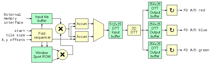
Figure 9. MCLT converter for the Bayer mosaic tiles
MCLT converter for the Bayer Mosaic data shown in Figure 9 is similar to the already described converter for the monochrome data. The first difference is that now the Fold sequencer addresses larger source tiles – it is run-time configurable to be 16×16, 18×18, 20×20 or 22×22 pixels. Each tile may have different size – this functionality can be used to optimize external memory access: use smaller tiles in the center areas of the sensor with lower lateral chromatic aberrations, read larger tiles in the peripheral areas with higher aberrations. The extended tile should accommodate all three color shifted 16×16 blocks as illustrated in Figure 10.

Figure 10. Example color channels 16×16 pixel tiles mismatch due to the chromatic aberration
The start input triggers calculation of all 3 colors, it can appear either each 256-th clock cycle or it needs to wait for at least 16 cycles after the end of the previous tile input if started asynchronously. X/Y offsets are provided individually for each color channel and they are stored in a register file inside the module, the integer top-left corner offset is provided separately for each color to simplify internal calculations.
Dual-port window ROM is the same as in the monochrome module, both horizontal and vertical window components are combined by a multiplier and then the result is multiplied by the pixel data received from the external memory buffer with configurable latency.
There are only two (instead the four for monochrome) accumulators required because each of the “folded” elements of the 8×8 DTT inputs has two contributor source pixels at most (for green color), while red and blue use just a single accumulator. Red color is processed first, then blue, and finally green. For the first ones only the DCT-IV/DCT-IV input data is prepared (in 64 clock cycles each), green color requires DST-IV/DCT-IV block additionally (128 clock cycles).
DTT output data goes to three parallel dual-port memory buffers. Red and blue channels each require just single 64-element array that later provides 4 different values in 4 clock cycles for horizontally and vertically flipped data. Green channel requires 2*64 element array. These buffers are filled one at a time (red, blue, green) and each of them feed corresponding phase rotator. Rotator outputs need 256 cycles to provide 4*64=256 FD values, the symmetry exploited during DTT conversion is lost at this stage. The three phase rotators can provide output addresses/data asynchronously or the green and blue outputs can be delayed and output simultaneously with the green channel, sharing the external memory addresses.
MCLT Converter for the Bayer Mosaic Tiles Simulation and Comparison to the Software Post-processing results

Figure 11. MCLT converter for the Bayer mosaic simulation
Results of the simulation of the MCLT converter are shown in Figure 11. Simulation ran with the clock frequency set to 100 MHz, the synthesized code should be able to run at at least 250 MHz in the Zynq SoC of the NC393 camera – at the same rate as is currently used for the data compression – all the memories and DSPs are fully buffered. Simulation show processing of the 3 tiles: two consecutive and the third one after a minimal pause. The data input was provided by the Java code that was written for the post-processing of the camera images, the same code generated intermediate results and the output of the MCLT conversion. Java used code involved double precision floating point calculations, while the RTL code is based on fixed-point calculations with the precision of the architecture DSP primitives, so there is no bit-to-bit match of the data, instead there is a difference that corresponds to the width of the used data words.
Results
The RTL code (licensed under GNU GPLv3+) developed for the MCLT-based frequency domain conversion of the Bayer color mosaic images uses almost the same resources as the monochrome image transformation for the tiles of the same size – three times less than a full RGB image would require. Input window function modification that accounts for the two-dimensional fractional pixel shift and the post-transform phase rotators allow to avoid re-sampling for the image rectification that degrades sub-pixel resolution.
This module is simulated with Icarus Verilog (a free software simulator), results are compared to those of the software post-processing used for the 3-d scene reconstruction of multiple image sets, described in the “Long range multi-view stereo camera with 4 sensors” post.
The MCLT module for the Bayer color mosaic images is not yet tested in the FPGA of the camera – it needs more companion code to implement a full processing chain that will generate disparity space images (DSI) required for the real-time 3d scene reconstruction and/or output of the aberration-corrected image textures. But it constitutes a critical part of the Tile Processor project and brings the overall system completion closer.
References
[1] Thiébaut, Éric, et al. “Spatially variant PSF modeling and image deblurring.” SPIE Astronomical Telescopes+ Instrumentation. International Society for Optics and Photonics, 2016. pdf
[2] Řeřábek, M., and P. Pata. “The space variant PSF for deconvolution of wide-field astronomical images.” SPIE Astronomical Telescopes+ Instrumentation. International Society for Optics and Photonics, 2008.pdf
[3] Malvar, Henrique. “A modulated complex lapped transform and its applications to audio processing.” Acoustics, Speech, and Signal Processing, 1999. Proceedings., 1999 IEEE International Conference on. Vol. 3. IEEE, 1999.pdf
[4] Britanak, Vladimir, Patrick C. Yip, and Kamisetty Ramamohan Rao. Discrete cosine and sine transforms: general properties, fast algorithms and integer approximations. Academic Press, 2010.
Leave a Reply