Elphel Development Blog

“Zoom in. Now… enhance.” – a practical implementation of the aberration measurement and correction in a digital camera

This post describes the implementation of the optical aberration measurement and correction developed for Elphel Eyesis cameras, the same methods and the code (available under GNU GPLv3) can be applied to many other camera systems. With 1/2.5″ 5 megapixel sensor we achieved average sharpness improvement over the image area around 40% compared to the raw images, effectively doubling the resolved pixel count. The applied correction varied significantly with the location on the image plane, orientation and color channel, making simple uniform isotropic sharpening (i.e. with “unsharp mask” or similar filtering) useless in our case. The aberrations correction is based on well-known measurement and inversion of the system point-spread function (PSF), additionally we describe used frequency domain de-mosaic filtering (“spectral scissors”) compatible with the inverted PSF convolution.

The sensor resolution and the lens resolution

Image sensors are improving in resolution, in the small format sensors this progress is boosted primarily by the cellphone cameras applications. When we just started Elphel in 2001 the 640×480 was considered “high resolution” for the C/CS-mount lenses so finding a good lens for even 1.3MPix sensor was not easy then. For some time it was possible to use high quality 35mm format lenses (with appropriate adapters) to match the sensor resolution, but as the sensors progressed toward smaller pixel size that approach was not usable any more – the large lenses were following designs for the film and their lp/mm (line pairs per millimetres) were insufficient for the new small-pixel sensors, even as the overall “megapixels” of those lenses were larger than those of the sensors. For the 35mm format lens (36mm x 24mm full frame) to work as “5 megapixel” for the 1/2.5″ format 5MPix sensor with 2.2μ x 2.2μ square pixels it should be rated as “200 megapixels” because the image area of the sensor is 40 times smaller than that of a lens. I hoped that the availability of the small high resolution sensors would stimulate the development of the appropriate lenses, an of course advances in the sensor technology lead to the availability of the suitable lenses. But the sensors progress faster and the lenses lag behind.

In earlier days (especially for the larger format digital cameras that benefited from the good lenses available from the film advanced film cameras) it was common to use optical anti-aliasing (blurring) filters in the digital cameras to reduce color artifacts caused by the lenses producing images that were too sharp for then available sensors – now the situation is quite opposite. In parallel to the progress of the sensors the advance in the software color interpolation of the Bayer color mosaic took place, these algorithms are doing a good job of “guessing” the missing colors and reducing color artifacts without sacrificing the sharpness of the images.

Image sharpening and the panoramic applications

When the optical resolution is less than that of a sensor it is possible to apply some degree of image sharpening in the post-processing or inside the camera itself. There is a good description of the sharpening effects at Imatest web site. Such image enhancement can be done by different methods, i.e. convolving registered image with a small kernel, subtracting blurred copy of the original (unsharp mask). Normally such process uses the same filter for the whole image and it is calculated for the best result in the center area of the image and it is quite reasonable for most applications. Optically it is much easier to achieve best quality near the center of the image, our eyes too have the resolution dropping dramatically away from the center spot. In photography people got used to have good resolution, “focus” in the center, it is common to intentionally blur the background (i.e. using depth of field). Panoramic imaging applications are different, the overall resolution of the panorama is limited by the weakest link – the resolution near the margins of the individual images, areas where the composite image is stitched. When designing the Eyesis optical head we evaluated multiple lenses with focal length in the range of 4.5-5.0mm (calculated to have 8 sensors around in portrait mode) and they all had significant resolution degradation near the edges. Applying constant sharpening filter would not help much – if the filter was designed for the central sensor area (where the image quality was already good in our case) – the effect near the edges would be hardly noticeable. If it was made for the off-center – it would significantly over-sharpen image in the center producing unreasonably strong halos. To make things worse the required correction in the off-center areas normally has significant anisotropy , so the optimal sharpening for say top left corner of the image may make it worse when applied to the top-right corner: the image there would be over-sharpened in one direction and under-sharpened in the orthogonal one.

When starting the development of the image sharpening for the Eyesis camera we already knew that the camera needs variable correction over the image area (and the color components, of course) – the lens performance was studied earlier. We also found that there are significant individual variations between the different lens samples, so individual camera calibration would be required, we could not apply the same compensation data to the different cameras or camera sub-modules.

Convolution based correction of the image aberrations in the system

Measuring the lens performance and un-applying the effect of the optical aberrations is routinely used – one of the most known applications was “glasses” for the Hubble Space Telescope to compensate for the flaw in the main mirror. It is also commonly used in microscopy – in such application in most cases it is impossible to perfectly focus on the object as the depth of field is very small.

Using such method with consumer cameras is difficult for several reasons – lenses are often interchangeable, have iris, adjustable focus and zoom – each of these factors influence the overall aberrations of the system and would require re-measuring the aberrations that need to be known with great precision, otherwise “correction” can in fact make images even worse. Small format (and so small pixel size) sensors present an additional challenge of relatively high pixel shot noise which is unavoidably amplified when the aberration correction is applied; increased shot noise is caused by the small value of the pixel “full well capacity”.

On the other hand, when the lens is fixed, focus is not adjusted and there is no moveable iris in the lens (iris anyway has very little use for the small format high-resolution CMOS image sensors because of the diffraction limit and very large depth of field) it is possible to make individual calibration of the lens once and then apply the calculated correction to all subsequently acquired images.

Selecting test pattern for the PSF measurement

The first step to correct the lens aberration would be to precisely measure the point-spread function (PSF) of the system at different areas of the image. Then, if there are no zeros in the spatial frequencies area of interest it will be possible to inverse the the PSF and use the result to correct the image. At least to some extent limited by the PSF itself (no zeros – you can not compensate the loss at the frequencies that yield complete zero by multiplying), precision of the PSF measurement and the system noise (unfortunately rather high for the sensors with small pixels). Measuring PSF directly would require real point light sources – something that is common in astronomy where stars are perfect approximations of the ideal point sources with additional advantage that their locations are precisely known. In our case we need something brighter (long integration of the starlight will cause to much noise in the sensor if we would try to use stars among other problems). Small PSF size (still just few pixels wide in “bad” areas) combined with high pixel noise require different test targets.

What the test target should look like? The PSF is calculated by deconvolving the image data with the inverted ideal test pattern, it is done by calculating Fourier transforms of both, than dividing the result of the first (image) by that of a second (test pattern) and performing inverse Fourier transform. For this operation to be successful the test pattern needs to meet the following requirements:

1. It should have all the spatial frequencies of interest included
2. The pattern should be easy to detect in the image even when image geometric distortions are present
3. The period of the pattern (if it is periodic) should be large enough so the measured PSF instances would not overlap
4. The period of the pattern should be small enough so the PSF measurement grid (image plane points at which the aberrations are measured) will have sufficient resolution
5. Different phases of the pattern crossing pixels will be uniformly distributed so the sub-pixel resolution could be achieved

The first requirement is needed because otherwise we’ll have to divide zeros by zeros or at least very small numbers by very small numbers with the results being buried in the noise. It is OK to have some zeros, but the non-zero values should cover most of the spectral area without large gaps.

The second requirement is important as in the calculations we need to know precisely what is the ideal image that sensor sees after the aberration is applied. Keeping precise and known orientation of the target and the camera is not practical, additionally the image is subject to the image geometrical distortions, and we need to know the image without aberration with a sub-pixel resolution. With the pattern built on a regular periodic grid it should be not so difficult for the software to “recognize” that pattern even in the presence of the geometric distortion and locally compensate that distortion so the simulated (model) image will match the measured one to a fraction of a pixel precision. And stay so over the large enough area to be able to make reliable measurements even in the presence of some noise.

When using the periodic (or actually close to periodic, as distortion breaks the exact periods) pattern and calculating PSF, there would be PSF clones with the same period as the grid itself, because(when neglecting distortions) there is no way to tell which of the object grid cells was recorded as which pattern cell on the image. And so the “wings” of the PSF instances should be far enough to prevent overlapping, so that defines the minimal period of the pattern grid.

On the other hand we can not make the cells too big, otherwise the PSF measurement itself will not have enough resolution – the PSF varies along the image area and so we have to know it in all those locations, that puts an upper limit on the pattern grid period.

Last requirement is similar to that described in ISO 12233 about measuring the spatial frequency response (SFR) to get resolution higher than a pixel by following the black/white edge that crosses pixel grid at different distances from the pixels centers – short description of such measurements is in the page about SE-MTF ImageJ plugin.

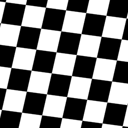
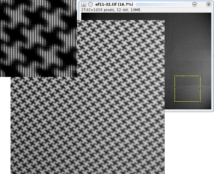
I started with the slanted checker board pattern – it was easy to recognize in the registered image and easy to generate the model that had the same local geometric distortions. Local distortions were approximated by the second degree polynomials and measured by finding the pattern phases in half-sized areas inside the full selection – full selection was 512×512 sensor pixels (256 x 256 for individual Bayer components), so that there were 128×128 squares in the center and shifted by 64 pixels in 8 directions.

Slanted checker board pattern

Windowed checker board pattern

Power spectrum of the checker board pattern

Filtered spectrum of the checker board pattern

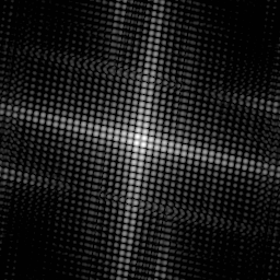
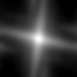
After working with such pattern for some time I realized that it had a major flaw – the spectrum was very anisotropic – 2 lines forming a tilted cross that extended to very high frequencies (even rolling over the margins) while having very little energy between those directions. The net effect of such anisotropy was that the lack of data in the “dark” areas of the power spectrum, the calculated PSF also had cross-like artifacts that I first tried to compensate in the code but that did not work well enough. It was possible to cut off the long legs of the cross, but boosting gain between them led to the increased noise and artifacts in the measured PSF.
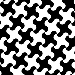
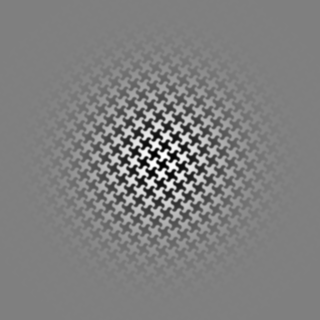
Then I tried to improve the pattern itself to reduce the anisotropy of the pattern spectrum while keeping it simple to generate and detect in the images, preserving the “inversion” feature of the plain checker board: if the pattern is shifted by one cell in either direction it becomes it’s own negative – white cells are replaced by the same shaped black ones and vice versa. The pattern was generated by replacing the straight sides of the squares with a pair of equal arcs, so the squares had circular segments added/removed. Such patterns worked much better – the calculated PSF did not have the artifacts without any additional tweaking, at the same time even the unmodified code could recognize the pattern in the image and calculate the grid parameters to generate a simulated model that matches measured data.

Curved pattern

Windowed curved pattern

Power spectrum of the curved pattern

Filtered spectrum of the curved pattern

Acquiring and processing of the target pattern images

The camera lenses are focused at approximately 9-10 meters so the depth of field for the selected lenses would extend from the infinity to – to as close as possible, that is about 6 meters. Using the test pattern even at 6 meters that would cover all the sensor would require about 5m x 7m target that is rather difficult to make and use in our office, so the software is designed to be able to combine measurements from the multiple frames, each having pattern covering only part of the sensor image area. Temporarily for the software development we used full pattern at just 2.25meters from the camera; with that distance the red (not the green) color is in-focus because of the axial chromatic aberration – that will be visible later from the PSF (and MTF) plots.
All 3 color components are processed individually through most of the chain, the corrected images are only combined at the very last stage. So the first step after acquiring the pattern image from the camera and transforming it into linear Bayer mosaic is splitting it into individual arrays

At this stage only the green color component is used for measuring the distortions, the dispersion of distortions is considered small, so even as the grid in different colors may have some shift, these color grids could be (locally) matched by translation to the sufficient precision. Both green components of the Bayer mosaic are combined here into a single square array of pixels rotated by 45 degrees from the sensor pixel array. The area that will later be used for PSF measurement is divided in smaller ones and for each the linear grid parameters are calculated.
These parameters include 2 wave vectors (2 numbers each) and 2 phases that define the grid at any point of the image in linear approximation. This is done by multiplying green pixels array by a Hamming window function, calculating power spectrum and then calculating the autocorrelation of this power spectrum. The result is a smooth pattern that is used to determine the wave vectors parameters of the image pattern, it is clusterised, and each cluster is verified to lay on the same line with equal distances from the previous ones. Then centroids of the pixels inside each cluster are calculated and combined resulting in the two vectors. That data is applied to the complex spectrum of the original image pattern to determine the grid phases. These values calculated on a 3×3 grid of samples allow to determine the second degree polynomials that describe local grid distortions. Knowledge of these coefficients allows to generate a model pattern that matches the recorded image with a sub-pixel precision.

Spectrum of the green component pixels

Autocorrelation of pattern spectrum amplitudes

Clusters found on the autocorrelation of the pattern amplitude spectrums

Upsampling the color component data

While the simulated pattern can be calculated to any resolution, the sensor data is not, of course. The lens aberrations can still be measured with higher-than-pixel resolution. It is so because we can process multiple periods of the pattern grid with the pattern cells and the cells have near-random phases with respect to the pixel grid, it is similar to the use of the slanted edge technique where the crossing points on different scan lines have different pixel phases. That extra resolution in the PSF (and later – inverted PSF kernels for convolution with the raw images) is really desirable. For example, if we have very sharp images, but one color is shifted half-pixel lateral chromatic aberration, there is no way to represent it without the significant blur. If the recorded line pixels are 0,0,1,0,0 then the chromatic-corrected would be 0,0,0.5,0.5,0 – the “point” becomes twice wider. Of course, it is an extreme case, and the input sequence would be already wider than one pixel, but for the good lenses – not much wider. Then wasting 1/2 pixel width of the sharpness would be a considerable loss, especially if we recall that the color component arrays have 1/2 resolution for red and blue colors and 1/sqrt(2) for the green one. So in this work I used 2x upsampling of the sensor pixels, that becomes 4x upsampling for red and blue components and 2*sqrt(2)~=3x for the green.
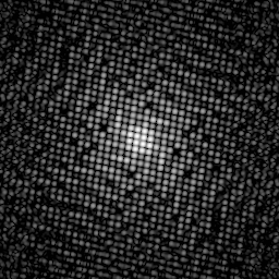
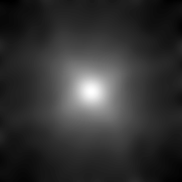
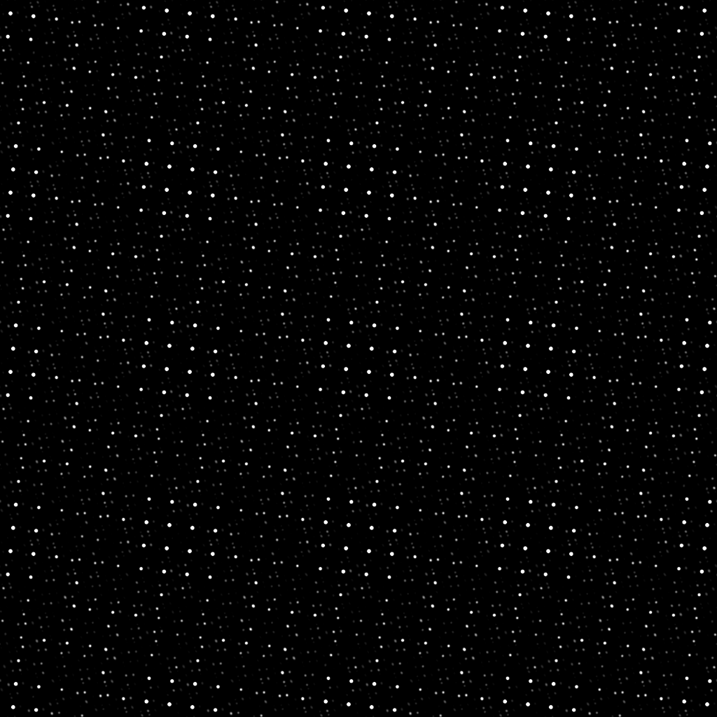
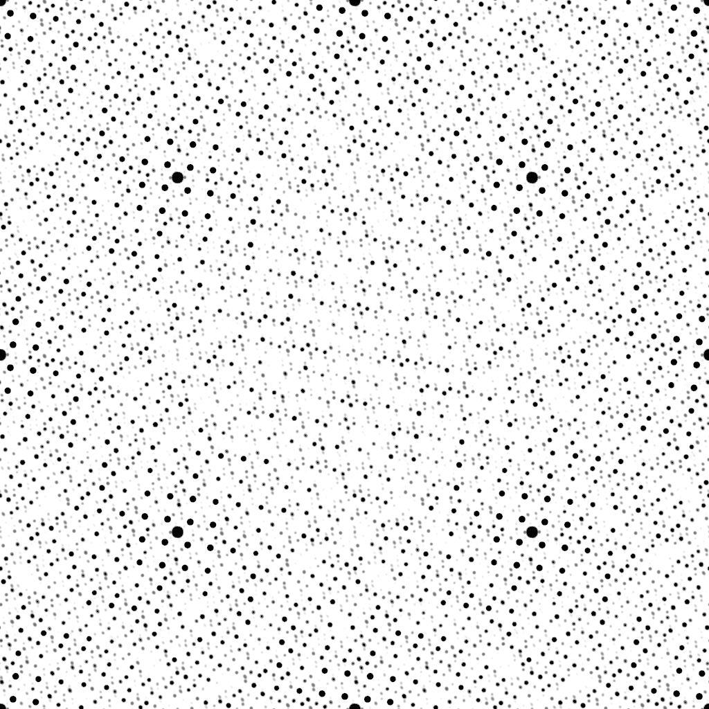
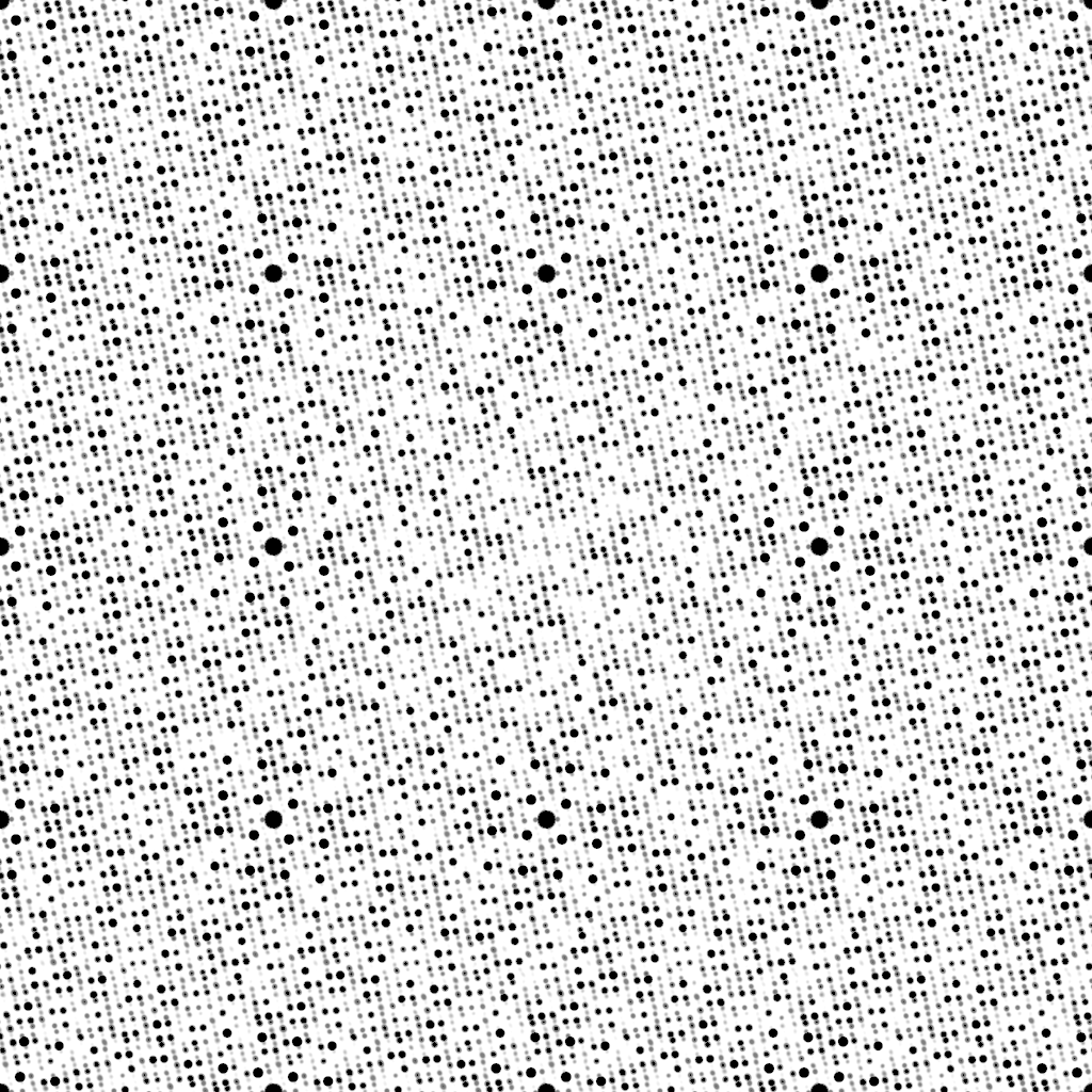
The power spectrum of the simulated pattern (it has some Gaussian blur applied to limit the spectrum for clarity) consists of a grid of spots. The size of each spot is reverse proportional to the size of the widow, so the larger the processed area, the smaller would be the spots. The distances between the spots (they lay on a 2-d parallel grid) represent the frequencies of the source pattern – the smaller the pattern cells, the farther would be the spots. The spots closest to the center represent the longest sine waves that go through black-white-black adjacent cells in the pattern, number of spots that would fit on a line from side to side would be the pattern period in pixels. So the ratio between the inter-spot distance and the spot size is the number of the pattern periods that fit in the processed area (multiplied by the window function). We can not make pattern period too small to avoid overlapping of the PSF instances (it should be several times larger than the worst blurring) and can not make the processing area too large it would cause low resolution grid of the PSF samples.

Simulated pattern with applied distortions with 1/2 sensor pixel resolution, blurred

Power spectrum of the simulated pattern

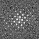
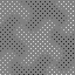
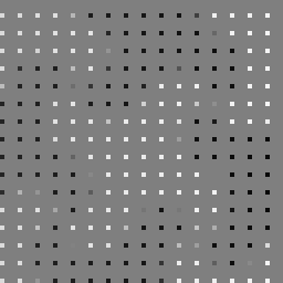
What happens to the spectrum when pixel sampling is applied and most (15/16 for red/blue and 7/8 for the green) pixel data is lost (zeroed out here)? There appear identical clones of the “ideal” spectrum – 7 for the green pixels (the function is periodic with the roll-over at top/bottom and right/left edges) and 15 clones for the red and blue colors.

Green pixels pattern sampled at half-pixel grid, enlarged fragment

Green pixels pattern, amplitude of the spectrum

With the Gaussian blur applied to the original (before downsampling) pattern there is very little overlap in the case of the green pattern but there is more of that in the case of higher degree of downsampling for the red and blue channels where it is difficult to distinguish between the spots that belong to the main instance and those that belong to the clones caused by the pixel decimation. But if the spots are small (relative to the distance between them) there is a good chance that it would be possible to distinguish the source of most of the spots. “Chance” is used here because of the image distortions the patterns for different areas of the image area are slightly different and so are the overlaps.

Red pixels pattern sampled at half-pixel grid, enlarged fragment

Red pixels pattern, amplitude of the specrum

The power spectra of the model (that do not have aliases) are used to generate filters to be applied to the OTF (optical transfer functions) of the registered images using the following procedure: they are duplicated and shifted (with periodic roll-over) according to the locations of all the aliases (excluding the main instance), 15 times for the red and blue color components and 7 times for the green ones. The results are accumulated into three arrays (one per color component) and discriminated using two threshold values – all elements below the lower threshold resulted in the value of 1.0, all the others above the high threshold – 0.0, with the smooth transition between the two values. These 3 masks were used to completely remove all of the the sampling aliases from the images of the test pattern – contrary to the de-mosaicing of the the live images (discussed later) the registered images of the known test patterns (after the proper distortion correction) have exactly known locations of the maximums on the power spectra as long as the detection process can be considered linear. The linearity is provided by using binary colors (just black and white, no greys that could produce different results depending on the printing process and illumination conditions) and un-applying known gamma-correction of the camera

Mask to reduce influence of the spectral clones caused by decimation (green color)

Mask to reduce influence of the spectral clones caused by decimation (red and blue colors)

Having Fourier transform of the simulated pattern that matches the image, Fourier transform of the upsampled image color components and the clone rejecting mask, it is now possible to calculate the PSF for the selected area of the system. After dividing the Fourier transform of the acquired image by that of the simulated pattern, multiplying the result by just calculated mask and performing inverse Fourier transform we are supposed to obtain the needed result.

Additional step is needed to make the this procedure work – the zeros and just areas where the model spectrum (denominator) has low amplitude would provide high values after division – unavoidable noise in the measured data would result in non-zero values in the nominator. Division would produce rather random high values and the inverse FFT would result in the useful signal being buried under the random patterns. This can be handled by imposing the lower limit on the denominator amplitude, and the current software uses x/(x²+a) function instead of just 1/x for the amplitude of the inverted denominator.
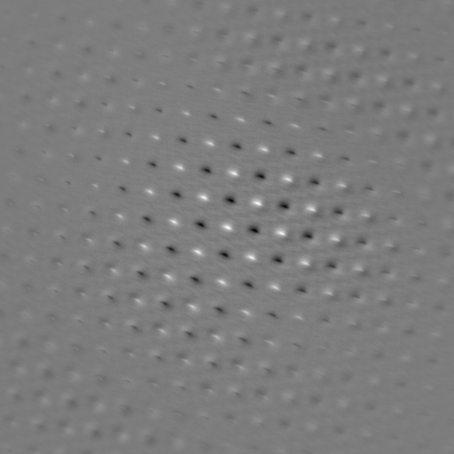
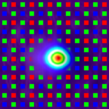
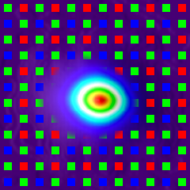
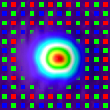
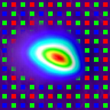
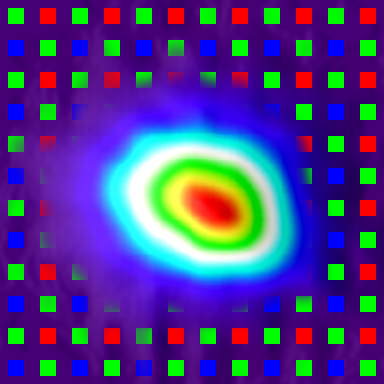
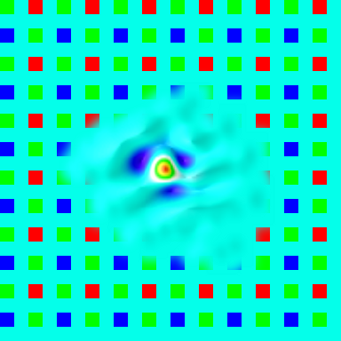
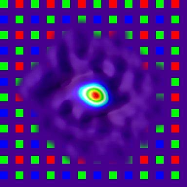
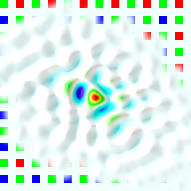
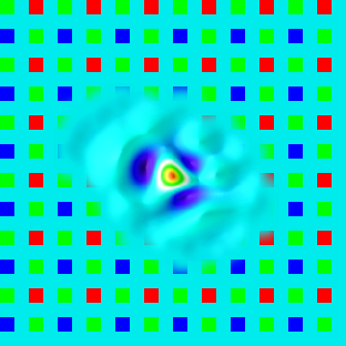
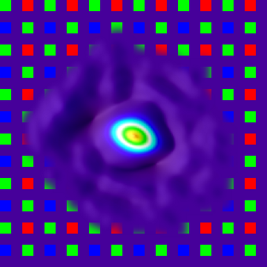
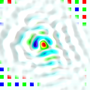
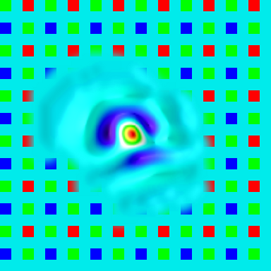
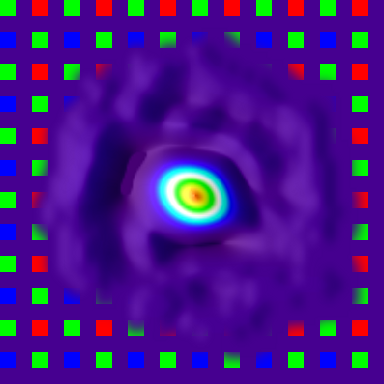
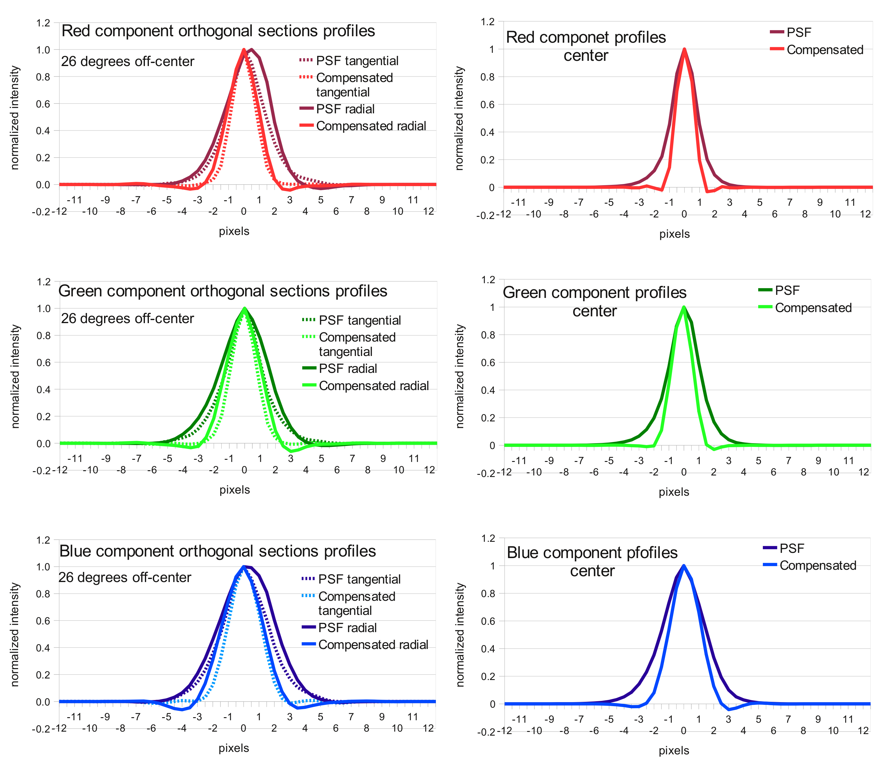
When the division is restricted in such way, deconvolution produces expected results like shown on the illustration where there is a grid of positive and negative PSF instances, sharp and high-contrast near the center and fading and blurring towards edges. Negative instances appear when acquired and simulated patterns are shifted half-period and black cells on one match equal white ones on the other. Degrading of the PSF instances when moving from the center is caused by distortions: the pattern approximately matches itself when shifted by 1/2 or one period, but the farther the patterns are moved, the less they match, because they are not strictly periodic, only approximate. In the next step some center instances (selected by comparison of the ratio of the instance contrast to the contrast of the center instance and the programmable parameter) are combined to farther reduce random noise. The results of the measurement of the PSF in the center and 26° off-center are presented in pseudo-colors with white color band corresponding to the intensity level of 50% of the maximal.

Measured PSF in the center and at 26° off-center, shown on top of sensor Bayer mosaic for the scale. White color band corresponds to 50% of the maximal value

PSF red, center	PSF green, center	PSF blue, center
PSF red, 26°	PSF green, 26°	PSF blue, 26°

Calculating an inverted PSF

When the PSF is measured for all the color components, all the image areas it is a tool to evaluate the lens performance. It is now possible to calculate the derivative parameters of the camera Spatial Frequency Response (SFR) such as Optical Transfer Function (OTF) and it’s amplitude – Modulation Transfer Function (MTF). Additional steps are needed to use this data for the enhancement of the image sharpness. When the PSF is just inverted (even with removing areas around zeros on the SFR), the inverted PSF has multiple oscillations extending far from the center. If such kernel is convolved with the raw image it amplifies the noise in that image and can completely bury the useful data. Some noise increase is intrinsic to this method (as other sharpness enhancement ones) but we need to maintain a careful trade-off between the amount of noise and the sharpness, not adding the noise without simultaneous increase in sharpness. One of the basic ways to filter out insignificant (or caused by the measurement noise) components is to apply combined spatial-frequency filtering or apodization so the the high spatial frequencies are preserved in the center area, but gradually filtered out in the areas farther away. In most practical cases (not to count special cases, like out of focus images with distinct bokeh) actual PSF has highest frequency components localized near the center of the PSF, while the noise signal covers all the area uniformly (you can see some small waves near the foot of the PSF shown above especially in “PSF blue, 26°”).

The processed image is calculated by convolving the original image with the calculated kernel, each result pixel is made of a sum of input samples multiplied by the elements of the kernel array. With the low contrast images the noise in each pixel (prevailing is the shot noise) is approximately the same, and as this noise is un-correlated between the pixels, it adds up as squared values of the elements. At the same time, the sum of kernel elements (some are negative) is the same as the DC gain and so is equal to one (1.0). Unity value of the DC gain means that levels of large areas of the same pixel values should yield the same value after correction, so it is possible to estimate the noise gain by calculating the square root of sum of squared kernel elements, and the kernels with multiple oscillations changing sign of the kernel elements result in higher output noise than those with less number/amplitude of oscillations.

Probably some wavelet-based processing could produce such filtering directly and be less computationally intensive than using the FFT-based processing, but here we implemented just a variable blurring equivalent to the Gaussian blur with the value of sigma being proportional to the distance from the kernel center. So as you can see on the illustrations, in the center the filtered kernels closely follow the originals but farther from the center the amplitude of oscillations falls off much faster. We also used the the other methods of filtering the result kernel amount of each defined by the setup parameters in the following order:

1. “Variable sigma” filtering of the PSF kernel as described above.
2. “Frequency modesty” filtering by approximating the OTF amplitude with an ellipse, scaling this ellipse and using it as a frequency domain mask. “Modesty” here means that we do not try to improve response on the spatial frequencies above certain value, proportional to the source system performance in that area, in that direction.
3. “Spatial modesty” filtering by approximating the direct PSF (spatial domain) with an ellipse, scaling it and using the result shape to generate a spatial window function for the result inverted PSF (calculated with inverse FFT of the filtered OTF). That limits the extents of the result kernels to be proportional to those of the PSF.
4. “Variable sigma” filtering of the inverted PSF kernel.

Inverted PSF red, 26°	Inverted filtered PSF red, 26°	PSF convolded with inverted filtered PSF red, 26°
Inverted PSF green, 26°	Inverted filtered PSF green, 26°	PSF convolved with inverted filtered PSF green, 26°
inverted PSF blue, 26°	Inverted filtered PSF blue, 26°	PSF convolved with inverted filtered PSF blue, 26°

When the filtered inverted PSF function is convolved with the measured PSF you could not expect to get an ideal delta function – such would be a result of convolution with the full spatial frequency range, unfiltered array. But that output would depend on minor fluctuations in the input data, mostly caused by the measurement errors, noise. So when applied to actual images or just independently measured PSF that nice result would fall apart. So instead of all pixel zeros but the center point, convolution provides some “sharper” that the original functions – about 1.45 times sharper for the off-center pixels if we compare full-width half-maximum (FWHM) values for different colors. That is not extremely large gain, but if we compare “megapixels” that are commonly used to benchmark both the sensors and the lenses used with them, the ratio is proportional to the square of the PSF FWHM value and it reaches 2.1 in that example, so potentially we can double the effective “megapixels” of the camera.

	PSF FWHM (pix.)	Compensated PSF FWHM (pix.)	FWHM ratio
Red, center	1.7	1.31	1.3
Red, 26 degrees, tangential	2.85	1.89	1.51
Red, 26 degrees, radial	3.37	2.15	1.57
Green, center	1.93	1.61	1.2
Green, 26 degrees, tangential	2.64	1.83	1.44
Green, 26 degrees, radial	3.48	2.47	1.41
Blue, center	3.16	2.17	1.45
Blue, 26 degrees, tangential	3.34	2.46	1.36
Blue, 26 degrees, radial	4.45	3.2	1.39

Frequency-domain image de-mosaic processing

Having the deconvolution kernels measured it could be apply them to the actual images and see the sharpness improvement, but the camera provides the Bayer mosaic output. Normally that data should be subject to some of the advanced de-mosaic algorithms that guesses the missing color pixels. Most of them rely on the fact that the sensor receives optically “ideal” image and sharp black/white edge would cross the pixel array as if the array was monochrome. In the case when optical aberrations are present that is not the case and we need an algorithm that does not require precise spatial matching of the color components of the image on the sensor, and for each area that is large enough compared to the PSF size the de-mosaic processing should be preferably represented as a linear filter, or convolution with some kernel. In that case we can apply both de-mosaic and sharpening to each individual color component and combine them later.

The simplest de-mosaic filter is just a low-pass filter (i.e. Gaussian) that averages values in some vicinity and so fills the missing pixel values, so I started with exactly that. But of course that causes decrease of the image sharpness and sensor resolution is not yet dramatically higher than that of the lens, so a better (locally linear) de-mosaic algorithm was needed. There is a good overview and comparison of the different demosaicing methods (including the frequency domain ones) in the work by Xin Lia, Bahadir Gunturkb and Lei Zhang Image Demosaicing: A Systematic Survey, here we used rather simple one that meets our requirements of being a locally equivalent to a set of the linear filter for the color components

Image below show different stages of processing of the model image – that image was made of a fraction of the letter “W” (its bottom-left part) that was slightly blurred and multiplied by a cosine-based window function – the same one that was used for processing of the actual images with 50% overlapping 64x64pixel tiles (corresponding to 32×32 sensor real pixels). The top left tile shows the monochrome original, in the top right corner there are 2 of the 3 sensor color component mosaic outputs – blue channel is similar to the red one and is processed in the same way. Contrary to the power spectra of the normal 2×2 Bayer cell, the images below are illustrating the up-sampled data (2x), matching the processing of the images prepared for the convolution. The source mosaic cell here is 4×4 with all the 12 pixels inserted into the original 2×2 cell assigned zero values.

This model image has two of the most common feature that are present in the real life images and various de-mosaic algorithms have to deal with. One is a linear border between light and dark (shown as “B”) and the other – a pair of the parallel borders of the opposite sign (wide line) – shown as “A”. Second image tile is the power spectrum of the source image, it is center (zero frequency) symmetrical as all Fourier transforms of the real (no imaginary part) input data. The linear border (as B) shows as a pair of the opposite “rays” perpendicular to the original border. The phase part of the Fourier transform depends on the location of the border in the image, but the amplitude does not – regardless of where that line is, the amplitude “ray” will start from the zero point. Pair of the opposite sign lines in the source (spatial) representation appear as an amplitude-modulated ray (as visible on “A”) – the closer the borders (narrower the line) the lower the frequency of the modulation would be.

Of course when we deal with the real image (not this model one) we do not have access either to the “source” image or to its spectrum, only to the sensor output (mosaics on the top right) and can calculate 2-d Fourier transforms of those (top middle, color corresponds to the pixel color). In that case the insufficient information from the sensor (missing pixels in the mosaics) lead to the appearance of the clones of the original spectra. In the case of the green components we have twice more (denser packaged) pixels than in the case of red (and blue) ones. And green spectra shows less of the clones, and out task is to separate the spectrum of the real image from those identical clones. If the source image is smooth, the spectrum would be narrow – small spot around the center, so the separation process would be simple – just cut the the circle around the center (zero) point with the radius about half of the distance to the center of the nearest clone – but that would be the low-pass filtering or “smoothing” that we already had to reject. The problem with the real life images that have distinct features with high-frequency components is that the their spectra extend far and overlap with those of the clones.

Next two rows show what happens with the isotropic (not relying on any image features) filtering. White dots mark the centers of the clones locations. Second row uses filtering with the radius of 1/2 of the distance to the nearest clone (larger in the case of green pixels as the clones are square root of 2 farter than for the red pixels). Columns 3 and 4 show the spectral amplitudes multiplied by the filter masks (columns 1,2) and the last (5,6) columns show the result of application of the same masks to the full (complex) frequency domain data and performing inverse Fourier transforms. As you can see the reconstructed images are blurred much more than the original, and still some artifacts are visible, and you can see that some parts of the clones spectra managed to get through even those narrow filters.

Third line shows similar filtering with 50% wider masks (3/4 of the distance to the nearest clone centers). Here most the “arms” of the center (true) spectra are preserved (so restored images are “sharper”) but much more of the unwanted clone parts went through, so the result images show excessive artifacts.

Last line shows the result of adaptive filtering that analyses the shape of the spectra and uses “scissors” to cut the spectral areas where clones dominate from the area with the high amplitude of the central (true) spectral instance. In the process of calculating the optimal shape of such cut we are using the fact that the spectra of different color components (especially in the high frequency areas) are close to each other and some degree of lateral chromatic aberration (mismatch of the colors) will not break this similarity. So we can use the shape of the green component spectrum (were clones are farther) to find the shape of the cut for the red/blue ones where the overlap with the clones is much higher. Some improvements to the currently used discrimination algorithm is possible – you can see that red component still let through some of the clone spectral components that got very close to the zero point that caused “wave”-like artifact on the red restored image, but it is visibly smaller than the default isotropic filtering produced.

The method used is aimed at detecting linear features (as shown with “A” and “B”), extending the preserved spectra along the rays for these features until they overlap with the clone power spectra. It involves conversion of the power spectrum to the polar coordinates array with the coordinates of the clones aliases prepared as an array of lists during the initialization. Then the filter area is expanded along the rays following the highest value of the power spectrum modified to detect modulated ones (FFT of the thick lines) until reaching the aliases. The full power spectrum is used when building the green filter; with the red/blue the power spectrum is multiplied by the green filter that was determined first.

Currently the green mask is applied to red and blue channels, but the data from the red and blue channels is not yet applied to the green one. Partially it is done so as in the distance range of interest of the Eyesis camera the optical resolution of the green channel is the best (even as it is not true for the currently used set of images, where the target distance was shorter than needed and red channel had the smallest PSF), partially – well, we just did not look into it yet. Most published works are using the test images recorded with the ideal lenses where the chromatic aberration amounts (both axial and lateral) are negligible. Additional work is needed to properly combine the de-mosaic and convolution-based aberration correction procedures.

The quality of the separation of the main spectra from the clones greatly depends on the orientation of the image linear features with respect to the sensor pixel grid. For example precisely vertical lines have spectral “rays” horizontal, and red/blue components have un-separable overlap even at rather low frequencies (same is true for the 45-degree lines and green component). As there are many vertical and horizontal lines in many images it may make sense to have sensors (or better yet mosaic patterns) tilted (i.e. 22.5°) so longer spectral “rays” are possible to separate from those of the clones.

Combining the processing steps

With the needed de-mosaic algorithm working it became possible to combine all the processing steps together and get the enhanced images. Actually at the time of this writing we did not yet print the full size test pattern images (the patter should be at least at 6 meters from the camera) so we were experimenting with the pattern at just 2.25m, and so the other images were made from approximately the same distance. We hope to have the larger pattern soon and to be able to process the real outdoor images acquired with the Eyesis camera.

The overall processing consists of the two parts – calibration (done once) and processing of each of the acquired images. Currently all the processing is implemented in Java as plugins for ImageJ, the per-image processing will be optimized for possible use of the GPU – it should be rather easy as most time-consuming parts are forward and inverse fast Fourier transforms (currently 128×128 for convolution and 64×64 for de-mosaic).

Calibration part involves

1. Measuring PSF for different parts of the image area,
2. Combining results from multiple images (otherwise we need about 5mx7m pattern that would not fit in out premises)
3. Interpolating PSF to the finer grid, matching the convolution kernel
4. Duplicating (or even extrapolating) PSF array to cover margins of the image – areas not covered in the measurement procedure
5. Inverting and filtering the interpolated PSF array

With the current implementations these steps take about 1.5 hours of the processing time per camera. This can definitely be optimized (originally the per-image processing was also running about that time) but it is not so critical – such calibration is required only once per camera.

Per image processing includes (times are for the processing on a one core of the 3GHz Intel I7 CPU):

1. splitting Bayer mosaic 2592×1936 image into color channels, upsampling it and adding margins around the image by replicating pixel patterns to reduce border effects during convolution using overlapping tiles – that process takes few seconds and results in 5248×3936 3-slice 32-bit images,
2. De-mosaic of the image using 64×64 tiles overlapped by 50% (32 pixels) – 50seconds
3. Convolving the result image with the inverted PSF kernel array – 108 seconds.
4. Convolving same image after de-mosaic processing with the Gaussian kernels having the same centers (lateral chromatic aberration correction) as the measured and inverted PSF, this is used for the processing of the smooth areas to reduce noise. This step can be optimized, currently it is the same computation as the previous step – 108 seconds
5. Combining results of 3 and 4 using threshold: areas with no details use the convolution with the Gaussian (resulting in less noise), areas with more high frequency components use “sharpened” image from step 4 – few seconds
6. Combining colors – converting to YCbCr, low-pass filtering of the color components and converting back to RGB. This step can be improved to better combine Y (intensity) channel from individual colors. Currently it also takes a few seconds.

Preliminary results

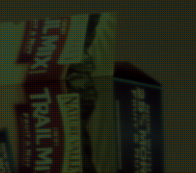
The illustrations below show small segments of the original and processed images, “full size” images that open when you click on the small ones below are scaled 4x from the original, the top left (dark) image shows the registered image as a mosaic of the color dots, corresponding to the actual sensor pixels. All the other images (but the VNG-interpolated produced by the external Ufraw program) are converted from the 3-component stacks to the color images using the same algorithm for comparison, during the normal processing only the final color stack is converted to color RGB image.

Second image in the top row shows the source image subject to a Gaussian blurring (and simultaneous lateral aberration correction). This image has the lowest sharpness but also the lowest noise – it is used in the areas where the amount of high spatial frequency is low. The rightmost image in the top row show the original processed by VNG (variable number of gradients) interpolation algorithm without additional sharpening.

The bottom left image shows the result of application of the frequency domain “spectral scissors” de-mosaic filtering. Next image the result of the deconvolution (sharpness enhancement) applied to that de-convolved image. While the sharpness is improved there is visible noise over the smooth areas (i.e. on the background). The last image combines the convolved one in all the areas where significant amount of high spatial frequency components is present, switching to the low sharpness/low noise in the smooth areas where the noise is most visible.

There is animated gif image – in is included near the top of the article that alternates between completely processed and just demosaiced images (same as bottom right and bottom left here). Another gif alternates between processed and de-mosaiced with a VNG, but as they were processed using different toolchain, the colors somewhat mismatch.

source image, Bayer mosaic (dark as most pixels are black)	source, convolved with the Gaussian kernel	source, processed with a standard VNG de-mosaic algorithm
Source, processed with frequency domain de-mosaic “scissors” algorithm	Source, convolved with the inverted PSF	Threshold-based combination of the convolution with the inverted PSF and the Gaussian (background areas)
Download archived GIMP file that combines these (scaled 4x) images as layers:processing-comparison.xcf_.tar.gz

The camera and the lens used for the described processing were not the top quality, we hope to be able to show the production images soon. The lens used so far was the one rejected for the Eyesis – we intentionally wanted to try software using the “worst case” optics, it had about 40% wider PSF than the lenses we use in the cameras. The test patter was much closer than the depth of field limit (2.25m instead of the 6m) as mentioned above, the camera itself was open combination of the sensor front end and the system board – same setup as used for the lens focusing. That left the sensor board open to the ambient light that resulted in the partially “washed out” image caused by the stray light. The software while being available for download from the very start of the development under the GNU GPLv3 free software license also needs some clean up (currently the main file is just some 15K lines of code) to become really useful for others, but please be assured it will not stay long in this state – we need it working efficiently and being easy to modify in the future.
Just following the release early, release often philosophy.