Elphel Development Blog

High Resolution Multi-View Stereo: Tile Processor and Convolutional Neural Network

Featured on Image Sensors World

This article describes our next steps that will continue the year-long research on high resolution multi-view stereo for long distance ranging and 3-D reconstruction. We plan to fuse the methods of high resolution images calibration and processing, already emulated functionality of the Tile Processor (TP), RTL code developed for its implementation and the Convolutional Neural Network (CNN). Compared to the CNN alone this approach promises over a hundred times reduction in the number of input features without sacrificing universality of the end-to-end processing. The TP part of the system is responsible for the high resolution aspects of the image acquisition (such as optical aberrations correction and image rectification), preserves deep sub-pixel super-resolution using efficient implementation of the 2-D linear transforms. Tile processor is free of any training, only a few hyperparameters define its operation, all the application-specific processing and “decision making” is delegated to the CNN.

Machine Learning for 3-D Scene Reconstruction

Machine learning is an active development area, and its applications to the 3-D scene reconstruction stimulated by the development of the autonomous vehicles including self-driving cars is no exception. Use of the CNNs to extract surfaces from the random-dot stereograms was published as early as 1992^[1]. Most of the modern researches use standard image sets: Middlebury stereo data set^[2] for high resolution near objects and KITTI^[3] for the longer range applications. KITTI images are acquired from a moving car, they have attached ground truth data captured by the LIDAR. This image set uses binocular pairs and has relatively low resolution (1.4 MPix) compared to the modern image sensors, and still most of the CNN architectures require from seconds to thousands of seconds even when implemented with GPU devices and so are not yet suitable for the real-time applications.

Most of the stereo image processing CNNs^[4] input raw pixel data and perform unary feature extraction in the parallel subnets (one for each image in a stereo set), merge features and perform additional processing of the resulting 3-D data. This is a so-called “siamese” network architecture that benefits from sharing parameters between the identical subnetworks. It is common to put most resources to the unary part of the processing resulting in truncating of the common stage of the processing that can consist of just a single layer (Fast Architecture in ^[4]). Efficient implementation in ^[5] limits CNN processing to just the DSI generation and then uses traditional methods of DSI enhancement such as semi-global matching^[6], other architectures split network after exchanging features and generate depth maps for each of the stereo images individually^[7].

Convolutional Neural Networks and the Frequency Domain Processing

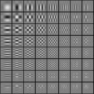
Early layers of the various CNNs (and the eye retina too) are very general and even remind the basis functions (Figure 2) of the two-dimensional Fourier (DFT), cosine/sine (DCT and DST) and wavelet (DWT) transforms so it is no surprise that there are works that explore combinations of such transforms and the neural networks. Some of them ^[8, 9] exploit the energy concentration property of these transforms that makes possible popular image compression such as JPEG. Others ^[10, 11] evaluate efficiency of the available Fast Fourier Transform implementations to speed-up convolutions by converting image data to the frequency domain and then applying the pointwise multiplication according to the convolution-multiplication property. Improvement is modest, as the frequency domain calculations are most efficient for the large windows, while most modern CNNs use small ones, such as 3×3, where Winograd algorithm is more efficient.

Tile Processor and the High Resolution Multi-View Camera

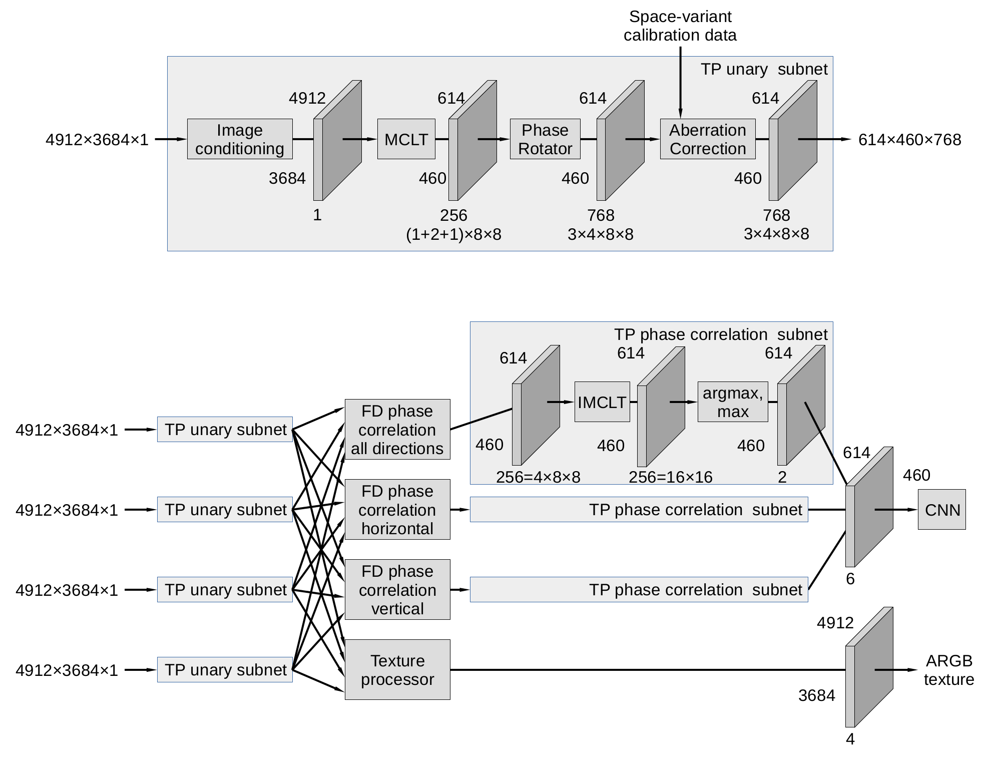
Multi-view high resolution cameras present a special case where frequency domain processing results may lead to the reduction of the CNN input features by two orders of magnitude compared to raw pixel input, the data flow diagram is presented in Figure 3. Four identical subnets process individual channels, each providing 4912×3684 pixel Bayer mosaic color images. As described in the earlier post Tile Processor is using efficient Modulated Complex Lapped Transform (MCLT) conversion of the Bayer mosaic (color) high resolution image data to the frequency domain, and of 4x8x8 coefficients representing full 16×16 input tiles for each of the 3 colors, red and blue result in 1x8x8 each, and green produces 2x8x8 coefficients, to the total of 256. Residual fractional pixel shifts needed for the image rectification are implemented as cosine/sine phase rotators, they are performed in parallel for each color and result in 768 coefficients for each tile. Frequency domain processing includes space-variant optical aberration correction (required for the high resolution small format image sensors), phase correlation for image pairs and textures processing if it is required in addition to the distance (disparity) measurement. Aberration correction is performed in each channel subnet, correlation and texture processing combine data from all four of them. After channels/pairs merging the frequency domain data is converted back to the pixel domain by the IMCLT modules as 16×16 tiles representing 2-D correlation. In most cases the 2-D correlation data is reduced to a 16-element array by summing perpendicular to disparity direction (orthogonal pairs are transposed in the frequency domain before they are combined and fed to the IMCLT), full 2-D correlation may still be used for the minor field calibration. The 16-element array is then processed to calculate sub-pixel argmax (residual disparity) and the corresponding correlation value (confidence) – this is where the number of features is dramatically reduced. It may be useful to increase the number of features and supplement average disparity for all 4 pairs of quad camera with separate horizontal and vertical pairs to improve foreground-background separation. These additional features are calculated by the identical TP phase correlation subnets as shown in Figure 3. With all 3 correlations each tile results in 6 values that are fed to the CNN input as a 614x460x6 tensor, in that case the feature reduction would still be over 40 (128 for a single correlation pair).

Conversion of the raw pixels to the Disparity Space Image (DSI) by the TP involves significant reduction of the (X,Y) resolution. When using four of the 18 MPix (4912×3684) imagers the result DSI resolution is just 614×460, this may seem like a waste of the sensor resolution. Actually, it is not:

• a deep sub-pixel resolution for disparity measurement needed for long-distance ranging requires matching of the large image areas anyway
• most of the image area for the most real-world images corresponds to smooth 3-D surfaces where assumption of a common disparity value for a tile is reasonable.
• the initial image resolution is preserved by the TP when source images are converted to the textures (simultaneously improving quality as the data from 4 rectified images is averaged)
• pixel-accurate distance map may be restored by extra processing the pixel data for selected tiles where depth discontinuity is detected, then assigning each pixel to one of the available surfaces.

Advantages of the TP+CNN over the End-to-End CNN

Significant (42..128) reduction of the input features is not the only advantage of the TP+CNN combination over the CNN alone. Being “convolutional” CNNs depend on translation symmetry, the groups of related pixels are treated the same way regardless of their localization in the image. That is only an approximation, especially when dealing with the high resolution images and extracting subpixel disparity values. This divergence from the strict convolution model is caused by the optical aberrations and distortions and requires use of the space-variant convolution instead, or performing complete aberration correction and image rectification before the images are fed to the network. Otherwise both the complexity of the network and amount of training data would increase dramatically. Image rectification with pixel (or slightly better) precision is a common task in stereo processing. It involves interpolation and re-sampling of the pixel data, the process that leads to the phase noise introduction, especially harmful when deep super-resolution of the matched images is required. Tile processor implementation combines multiple operations (fractional pixel image shifts, optical aberrations correction, phase correlation of the matched pairs), TP avoids image re-sampling from the sensor pixel grid by replacing it with the phase rotation in the frequency domain.

Final step that reduces the number of features that are sent from the TP to the CNN is extraction of the disparity value by calculation of the argmax of the phase correlation data. This function has to be calculated with subpixel resolution for the data defined on the integer pixel grid. Certain biases are possible, and the TP implementation offers trade-off between speed and accuracy. The result disparity value is a sum of the pre-applied disparity (implemented as a phase rotation in the frequency domain on top of the integer pixel shift) and the argmax value (correlation maximum offset from zero). When higher accuracy is required, a second iteration may be performed by applying the full disparity from the first iteration, then the residual argmax offset will be close to zero and less subject to bias.

System Performance Estimation and the Prototype Setup

Optimal system for the real-time high resolution 3-D scene reconstruction and ranging would require development of the application-specific SoC. If used with a set of four 18 MPix image sensors (such as ON Semiconductor AR1820HS) and a single ×16 1600 MHz DDR4 memory device, the 16 nm technology process, the TP subsystem will be capable of 10 Hz operation covering the full 4912×3684 frames reserving half of the memory bandwidth for other then TP operations.

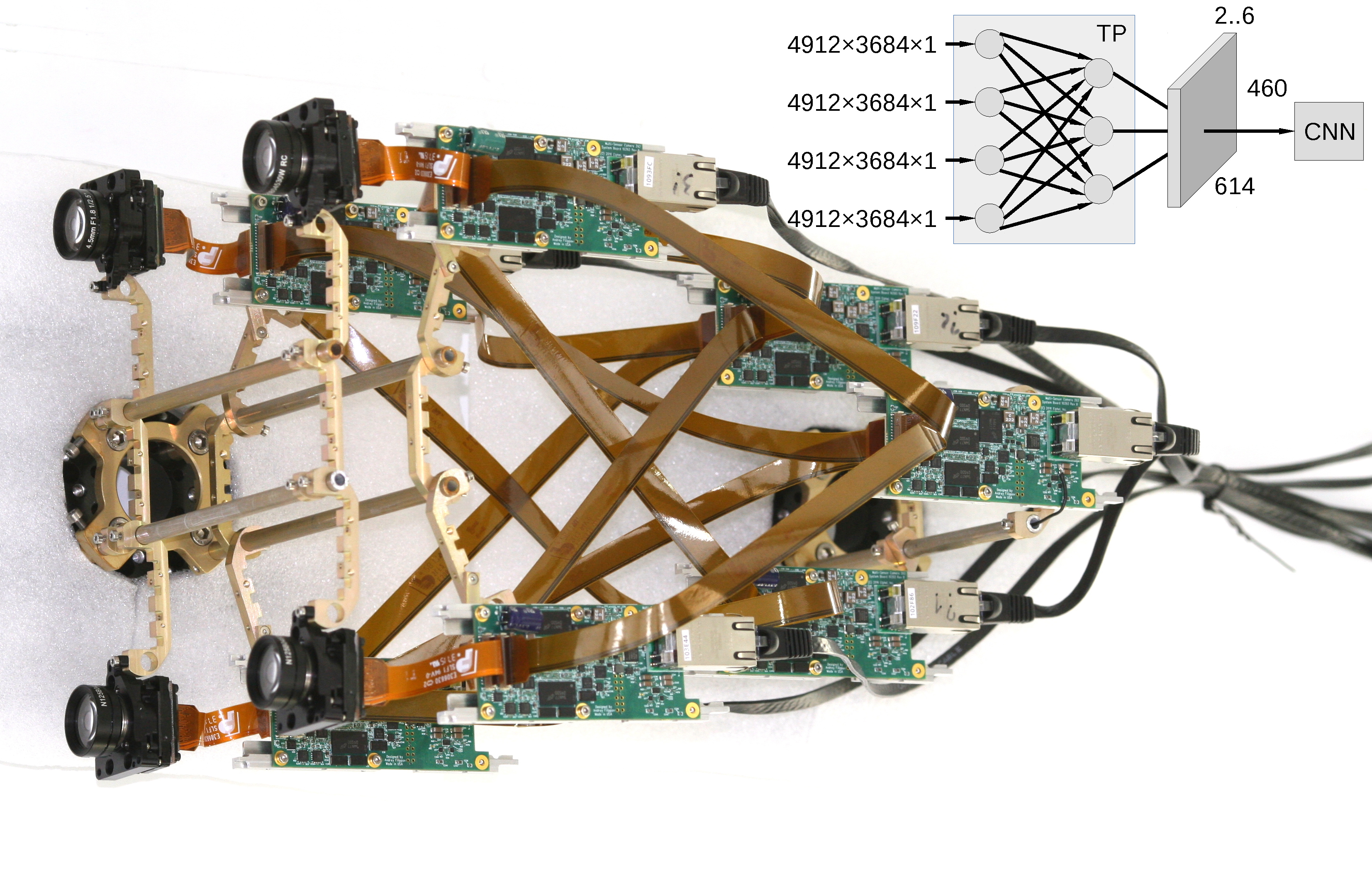
We plan to emulate such system using available NC393 camera electronic and optical-mechanical components, including multiple 10393 system boards based on Xilinx Zynq 7030 SoC. Each such board has a GigE port and four identical sensor ports routed directly to the FPGA I/O pads allowing flexible assignment of pin functions. Typical applications include up to 8 differential LVDS pairs, clock pair, I²C and clock input. The same connectors can be used for high-speed communication between the 10393 boards. Partitioning the system into multiple boards will allow to fit the required TP functionality into smaller FPGAs, then send the result features (614×460×6) over the GigE to a workstation with GPU for the experiments with different CNN implementations. The system bandwidth will be lower than that of the application-specific SoC, the 10 Hz operation will be possible with 5 MPix sensors (2.5 Hz with 18 MPix).

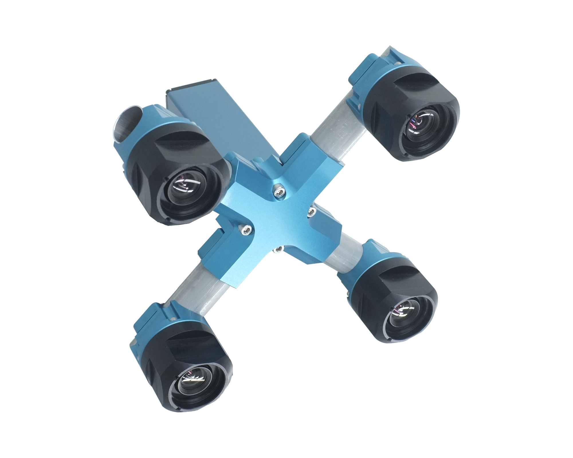
Inter-board connections are shown in Figure 1 (just the connections, the actual prototype camera will look more like in Figure 4, but with a wider body). Five to seven of the 10393 boards are arranged in 2 layers. Four layer 1 boards use one of the sensor ports to receive image data from the attached sensor, perform image conditioning, flat-field correction and store data in the dedicated DDR3 memory. They later read the data as 16×16 pixels overlapping tiles, calculate the tile centers using calibration data and requested location and nominal disparity from the data received over the GigE. Each tile is transformed to the frequency domain, the data is subject to the space-variant aberration correction. The result frequency domain tiles are output through three remaining sensor ports that are reconfigured to be LVDS transmitters. The layer 2 boards simultaneously receive frequency domain data through all 4 of their sensor ports from the layer 1 and perform phase correlation (pointwise multiplication followed by normalization) on the image pairs. There could be just a single layer 2 board, or up to 3 (limited by the available layer 1 ports) to perform different types of correlations in parallel (all 4 pairs combined, two vertical pairs and separately 2 horizontal pairs for better foreground/background separation. The results of the frequency domain calculations are then transformed to the pixel domain and the argmax is calculated. Then argmax value is used to calculate the full tile disparity, and the corresponding correlation value – as a disparity confidence. The pair (disparity, confidence) for each tile is then sent over GigE to the CNN implemented on a workstation computer.

Image Sets for Training and Testing

While the TP functionality is already tested with the software emulation, and the efficient implementation is developed, more research is needed for the CNN part of the system. Available image sets, such as KITTI^[3] have insufficient resolution (1.4 MPix) and they use different spatial arrangement of the cameras. We plan to capture high resolution quad camera image sets using available NC393-based cameras that will be upgraded from 5 MPix to 18 MPix sensors of the same 1/2.3″ format so the optical-mechanical design will remain the same. As we are primarily interested in long distance ranging (few hundreds to thousands meters), use of the LIDARs to capture ground truth data is not practical. Instead we plan to mount a pair of identical quad cameras (with the baseline of 150mm) on a car 1500 mm apart, pointed in the same direction, so when the 3-D measurements from these quad cameras are fused, the accuracy of the composite distance data would be ten times better, because the effective baseline will be 1500mm. Of course that method has some limitations (it will not help to improve data from the poorly textured objects) but it will provide higher absolute distance resolution that can be used for the loss function during CNN training. Data from the individual quad cameras will be used for training and testing of the network.

Update: here is the actual rig.

All acquired images, related calibration data and software will be available online under GNU GPL.

References

[1] Becker, Suzanna, and Geoffrey E. Hinton. “Self-organizing neural network that discovers surfaces in random-dot stereograms.” Nature 355.6356 (1992): 161.

[2] Scharstein, Daniel, et al. “High-resolution stereo datasets with subpixel-accurate ground truth.” German Conference on Pattern Recognition. Springer, Cham, 2014.

[3] Menze, Moritz, and Andreas Geiger. “Object scene flow for autonomous vehicles.” Proceedings of the IEEE Conference on Computer Vision and Pattern Recognition. 2015.

[4] J. Zbontar and Y. LeCun, “Stereo matching by training a convolutional neural network to compare image patches,” Journal of Machine Learning Research, vol. 17, no. 1-32, p. 2, 2016.

[5] W. Luo, A. G. Schwing, and R. Urtasun, “Efficient deep learning for stereo matching,” in Proceedings of the IEEE Conference on Computer Vision and Pattern Recognition, pp. 5695–5703, 2016.

[6] H. Hirschmuller, “Accurate and efficient stereo processing by semi-global matching and mutual information,” in Computer Vision and Pattern Recognition, 2005. CVPR 2005. IEEE Computer Society Conference on, vol. 2, pp. 807–814, IEEE, 2005.

[7] J A. Kendall, H. Martirosyan, S. Dasgupta, P. Henry, R. Kennedy, A. Bachrach, and A. Bry, “End-to-end learning of geometry and context for deep stereo regression,” arXiv preprint arXiv:1703.04309, 2017.

[8] Sihag, Saurabh, and Pranab Kumar Dutta. “Faster method for Deep Belief Network based Object classification using DWT.” arXiv preprint arXiv:1511.06276 (2015).

[9] Ulicny, Matej, and Rozenn Dahyot. “On using CNN with DCT based Image Data.” Proceedings of the 19th Irish Machine Vision and Image Processing conference IMVIP 2017

[10] Vasilache, Nicolas, et al. “Fast convolutional nets with fbfft: A GPU performance evaluation.” arXiv preprint arXiv:1412.7580 (2014).

[11] Lavin, Andrew, and Scott Gray. “Fast algorithms for convolutional neural networks.” Proceedings of the IEEE Conference on Computer Vision and Pattern Recognition. 2016.