Subpixel Registration and Distortion Measurement
Motivation
While working on the second generation of the Eyesis panoramic cameras, we decided to try go from capturing the series of the individual panoramic images to the 3d reconstruction. There are multiple successful implementations of such process, we just plan to achieve higher precision of capturing the 3d worlds using Elphel ability to design and build the hardware specific for such purpose. While most projects are designed to work with the standard off-the-shelf cameras, we are working on building the cameras together with the devices and methods for these cameras calibration. In order to be able to precisely determine the 3-d locations of the features registered with the cameras we plan first go as far as possible to precisely map each pixel of each sub-camera (of the composite camera) image to the ray in space. That would require at least two distinctive steps:
- map each pixel of each sub-image to the ray in the composite camera frame system and
- measure the composite camera egomotion to find the absolute pixels-to-rays mapping.
The first step can be done by calibration of the camera in the laboratory, measuring the position and orientation of each sub-camera relative to the composite camera frame and simultaneously measuring camera lens distortions. To implement the second step we plan to combine the inertial data from the high resolution/high bandwidth inertial measurement unit (IMU) with the optical data from the camera itself. This post is dedicated to the first part, the static pixel mapping of the composite camera.
The complete camera has 26 sub-camera modules and we are building a goniometer type camera calibration machine that will rotate the finished camera around two axes exposing the large calibration pattern (3.0m by 2.6m) to different areas of each of the sub-camera sensors. Registered images will be also used to correct each lens aberration as described in the earlier blog posts
Registering the pattern grid
We first designed the grid pattern for measuring (and correcting) the lens aberrations – it has less aliasing artifacts and more uniform spectrum than plain checkerboard pattern normally used for distortion measurement while still being easy to detect and register.
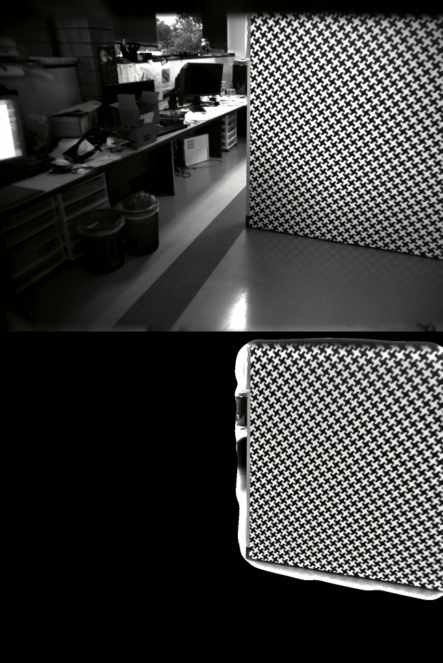
Processing starts from the Bayer mosaic image acquired from the camera and for distortion measurements only the green channel is used. Figure 1a shows the grid that occupies most of the image sensor area, other images may have the pattern in smaller areas, so the pattern registration starts with detecting pattern in at least some areas. For that the smaller (normally 128×128 pixels) square areas of green pixels are extracted as shown on Fig.1b the image is rotated 45 degrees from the original on fig.1a because green channel uses half of the sensor pixels, located in say “black” cells of the checker board pixel grid.
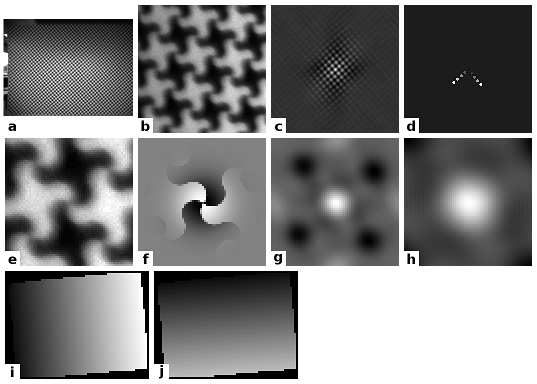
Fig.1 Pattern grid registration: a) registered image. b) 128pix*128pix region for green channels. c) power spectrum (gamma=0.2). d) clusters around first maximums in 2 directions. e) 64×64 region centered around the estimated grid node. f) simulated grid with window function applied. g) mixed cross/phase correlation of registered and simulated arrays. h) combination of correlations with 4 half-pixel shifted models. i) result pixel X coordinate for each of the registered grid nodes. j) same for the pixel Y coordinate
Next step is to calculate the spectrum of this pattern – Fig. 1c shows the power spectrum to the power of 0.2 to somewhat equalize the harmonics amplitude (it worked better than logarithm function). Pixel clusters around the first several maximums along the two pattern axes were extracted and used for initial measurement of the two pattern translation vectors (Fig. 1d). If no pattern is detected the scanning continues, instead of the sequential scanning I used reverse-bit order to reduce number of trials before hitting the area with the pattern.
After the program detects the first area with the pattern it continues with the more precise measurement of the correlation between the acquired image and the simulated pattern, calculated for the same grid translation vectors. Fig. 1e shows the 64×64 pixels fragment of the registered image centered around the estimated grid node (before multiplying by a window function) and Fig. 1f shows the matching simulated one with the window applied. Correlation is performed through direct and reverse Fourier transforms, run-time parameter allows changing from the cross-correlation to the phase correlation. Fig. 1g shows result of such operation applied to images on Fig. 1e and 1f.
While there is only one copy of the acquired image around the grid node shown on Fig. 1e, it is possible to generate the simulated image (Fig. 1f) with different sub-pixel shifts, combining the results of their correlation with the same source image can reduce effects of the aliasing and increase the resolution of the correlation result. The next image (Fig. 1h) shows the result of combining 4 of 64×64 pixels correlations where the simulated images are generated with 0 and 0.5 pixel shifts in each of the two directions, using the center 64×64 of the combined 128×128 image and application of a low-pass filter. This data is then used to calculate the coordinates of the grid node with one of the several methods – fitting the quadratic function or finding the centroid of the top of the maximum, cut at a specified threshold or area.
The whole process of calculating the locations of the grid nodes is ran twice. On the first pass program starts from the first node detected and uses the grid parameters to estimate the locations of the neighbor nodes and use this estimation to generate the local pattern simulation used for correlation. This process generates a wave from the initially detected point that propagates until all the connected grid nodes are processed and the correlation contrast (calculated as the ratio of the average signal inside the center circle and that in a ring that falls between the expected maximums) falls below the specified threshold. The program uses quadratic approximation for the simulated pattern generation to compensate for the local lens distortions – while not critical for the lens used in this work, that was important to fit the grid to the fisheye lens used in the first Eyesis camera.
The second pass refines the location of the grid nodes detected in the first pass – this time the locations of the neighbors already known are used for the local pattern grid generation. The result of this procedure is the array of grid points organized by the grid coordinates (u,v) with half of them (even sum of u+v) being “positive” and the other half (odd sum of u+v) being inverted. This data is stored as a multi-slice TIFF image, two of the slices: sensor pixel X coordinate and sensor pixel Y are shown on the Fig. 1i and Fig. 1j, respectively.
Evaluating results of the pattern registration
When several methods of pattern grid registration were implemented I needed some way to estimate the precision of the results, to be able to compare the influence of the different variable parameters (correlation size, window function, cross/phase correlation ratio) on this “registration quality”. Most interesting for us was how repetitive the registration results are so how their invariants would differ for the images acquired in at least approximately the same conditions.
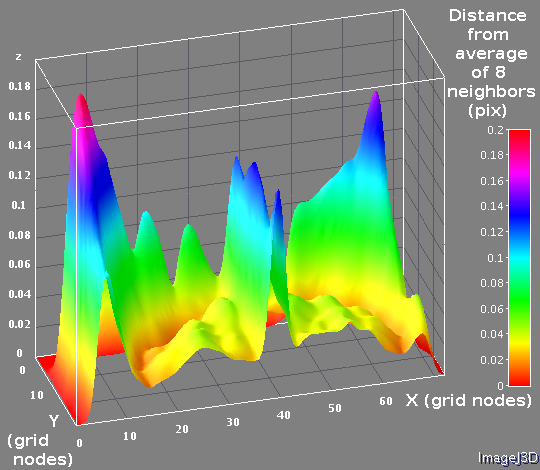
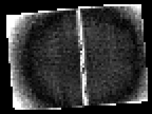
Fig. 2c Grid curvature – distance in pixels from the registered pattern grid node location and the average of it 8 neighbors. One half (corresponding to top of the Fig.2a) is shown.
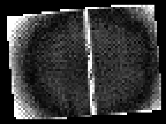
I used the following intra-frame estimate of the registration errors. First the program calculated the grid curvature as a difference between the selected grid node location (pixel X and Y values) and the average value calculated from the node neighbors. This value (shown on Fig. 2a-c) is dependent on the actual curvature of the registered grid (caused by the lens distortion), the errors of the physical pattern attached to the wall and the variations of the results of the registration method.
All of these three contributing factors reveal themselves on these images. The circular structures are related the optical distortions, the bright column in the middle of the Fig. 2a is caused by the small misalignment of the 2 halves of the physical pattern – it consists of the two 1.5m by 2.6m plastic panels attached to the wall. Each of the panels maybe (and actually is as we’ll see later) slightly distorted from the perfectly rectangular shape, and there is some error in alignment of the panels to each other.
There is also some “noise” visible on Fig. 2a (has to be smoothed out for 3d visualization on Fig.2c), and checker-board artifacts mostly visible near the corners of the images. These artifacts are likely caused by vignetting which has more effect on white parts of the pattern and so biases the registered location when the the overall brightness gradient coincides with the direction connecting the two opposite white quadrants of the pattern around the node. Vignetting correction that we’ll incorporate in the same measurement cycle will reduce this effect and improve the pattern grid node registration.
Update: yes, these artifacts were in fact caused by the lens vignetting and uneven illumination of the pattern. When the pattern images were equalized (see Fig. 2d) the artifacts were successfully eliminated (Fig. 2b). At this stage it is insignificant what causes the brightness gradients – lens or the light source, and the “flat-field” correction is only needed for the areas of the image where the test pattern is detected. The equalization is implemented after the first pass of of measuring the grid node coordinates. The program calculates average value of the pixels around these already known coordinates using the same window function as for the correlation. This method seems to work as is, but it can be improved to probe average pixel values around the estimated centers of white and black cells, in that case the result will less depend on the initial precision so it will work for lenses with higher distortions (as the fisheye ones).
When the average intensity is calculated for every known grid node, the border node values are removed because their value is influenced by the pixels outside of the pattern area. Next the average intensity map is expanded by extrapolating the measured intensity data outwards from the known cells to estimate the average intensity values near the pattern edges and beyond, so the low-pass filter would not skew the result. The average intensity map is then applied to the original image before refining the pattern grid node locations during the second pass (black area on Fig. 2d is not a privacy filter, it is just outside of extrapolation area ).
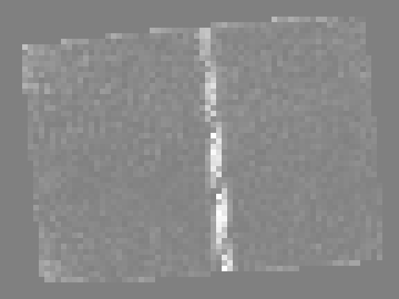
Fig.3a Registration errors as distances from the registered grid nodes to the calculated from the neighbors, assuming constant curvature. Full scale is 0.2 pixels
The high frequency variations on the Fig. 2a are caused by the registration errors – measurements described later did not show any detectable node-to-node differences on the pattern, only the gradual changes. To separate gradual variations caused by the lens and pattern distortions I subtracted the estimated (from the neighbor nodes) grid node location from the registered one, assuming the constant local curvature, the results are shown on Fig. 3a and 3b.
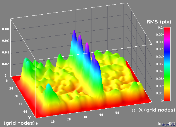
Fig.3b Registration errors as distances from the registered grid nodes to the calculated from the neighbors, assuming constant curvature.
The pattern discontinuity in the center is still present, but in the other areas the effects of the gradual variations are compensated. The checkerboard artifacts visible the Fig. 2a are hidden on Fig 3a, because the variations from the estimated (from the constant curvature) locations in these areas are opposite in direction, but same in length, so these artifacts just add to the average error value in the corners. The root mean square of these differences was used to compare different registration methods.
We plan to make more measurements of the registration errors with the complete multi-channel cameras when the precise rotation machine will be built, currently I used just a single camera mounted on a tripod.
Absolute mapping of the pattern grid with the laser pointers
The pattern grid registration procedure described above resulted in arrays of the pixel coordinates of the pattern grid nodes,but there was no information about the absolute position of the measured pattern cells relative to the pattern as a whole. In some cases when the corner of the whole pattern is visible and the approximate camera orientation is known (so one of the 4 corners can be identified) it is possible to make absolute mapping, but we decided to supplement the pattern with the four laser diodes pointed to the known cells in the four quadrants of the pattern. With the lasers controlled by the software it was easy to detect location of the laser spots by subtracting a pair of images (with and without the laser spot). The precision of the laser spot location is not critical as long as those spots safely identify known white cells of the pattern grid.
Absolute mapping of the pattern grid nodes is needed for both finding the extrinsic parameters of each sub-camera (position and orientation relative to the composite camera frame) and accounting for the non-ideal pattern grid when measuring the camera lens distortions.
Composite camera and the camera rotation machine combined model
Starting calibration of the composite camera I created a model to describe the location and orientation of each of the camera 26 sub-cameras relative to the composite camera frame, rotation of the composite camera in the calibration machine we are building (fixed horizontal rotation axis and moving camera vertical axis), deviations of the machine (distance between the axes, difference from the 90 degree angle between the axes, two angles to determine actual orientation of the horizontal rotation axis) and location of the machine reference point (point on the horizontal rotation axis closest to the camera rotation axis) relative to the frame attached to the target. Each of the sub-cameras is described by a set of 7 intrinsic parameters based on a radial distortion model (focal length, pixel coordinates of the lens axis and 4 coefficients describing distortion polynomial) and a pixel-mapped array to represent the difference from the radial distortion model.
The pattern grid is represented as a two-dimensional array (U,V) of the 3-d points. For the first experiments where all the images were acquired from approximately the same point the grid was considered flat (z=0), but the provision was made to store the full 3-d data for each pattern grid node to account for non-flatness of the physical pattern.
The composite camera is designed to capture all images at the same time and each of the result images is uniquely identified by a timestamp (common to all sub-cameras) and the sub-camera number. While only the sub-camera intrinsic parameters (7 with the selected radial distortion) and the 6 extrinsic ( 3 rotations and 3 translation) are sufficient to project each of the pattern grid points to the sensors I used a complete camera kinematic model to be able to impose constraints for the groups of images, such as that all the relative positions/orientations of the sub-cameras relative to the composite camera are common, all the parameters describing the calibration machine but the 2 variable rotations are also common, and these two variable angles are common for the images acquired from the different sub-cameras that share the same timestamp. Such model makes each image dependent on 15 extrinsic parameters and the conversion from 15 to 6 is common for each pattern node projection in the image.
The fitting of the parameters of the model to the series of pattern grid images is based on Levenberg-Marquardt algorithm (LMA) and the deviations to minimize are differences in X and Y directions between the calculated locations of the pattern nodes projections on the sensor and their registered locations. So each grid node on each registered image being processed constitutes two separate samples for the algorithm. This algorithm involves calculating Jacobian matrix of the partial derivatives. Most of the partial derivatives with respect to the minimal set of 7+6=13 parameters are different for each pattern node of each image, we do not need to calculate them for each of the 22 parameters because conversion from 22 to 13 (both values and partial derivatives) can be calculated once per image and then the Jacobian calculation for 22 parameters can be done by multiplying Jacobian for 13 parameters by the 22×13 matrix. The implementation of the LMA is designed to have sequences of programmable strategies, each specifying a subset of the grid images to process, set of parameters to adjust and if they are individual for each image, shared by all or by the groups of the images. Program can run strategies automatically or stop after each iteration step or one strategy series.
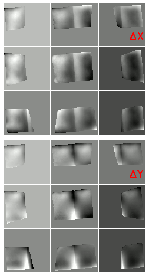
Fig. 5a Reprojection error of the pattern grid after fitting camera extrinsic parameters and the intrinsic ones assuming polynomial radial distortions, shown separately for X and Y directions. Full scale is +/- 2mm
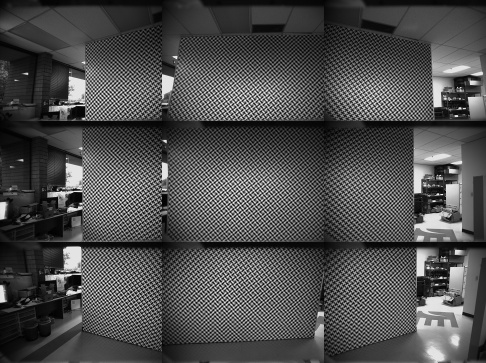
The experiment used a set of 15 images with a single camera mounted on a tripod at 2.3m from the pattern and rotated around approximately vertical axis to five positions in the range of ±30° for three different tilts in the range of ±15°. Nine of the 15 such images are shown on Fig. 4. The actual acquired images were already converted to the grid arrays and stored as multi-slice TIFF images as described above, so each new run of the program did not require re-running the pattern registration process. In addition to the two slices shown on Fig. 1e and 1f (pixel X and pixel Y coordinates) those files had additional slices of integer values U and V representing absolute grid coordinates of the same pattern nodes available after the absolute mapping with laser pointers.
Measuring the pattern geometry
Radial distortion model provides rather accurate projection of the pattern grid nodes to the image sensor pixel coordinates so I expected the physical pattern distortions (non-flatness and stretching of the material) to be the next source of mismatch between the model and the registered image, we’ve already seen them in the registration process as illustrated on Fig.2 and 3. And after I ran the LMA on a set of 15 images and it converged on parameter vector, I mapped the reprojection errors (differences between calculated and measured pixel coordinates) to the grid coordinates. The nine images of Fig. 5a (animated GIF) and Fig. 5b (color) match the acquired images shown on Fig.4, i.e. top left (of nine) image shows the top left portion of the pattern.
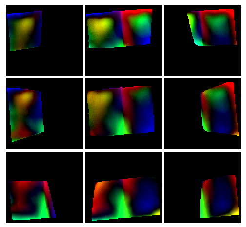
Fig. 5b Reprojection pattern grid errors in pseudo-colors. Different colors indicate different directions, brightness – the absolute value of the difference.
Each image frame on Fig. 5a and 5b represents the minimal straight rectangle that includes the full pattern, each sub-image covers different but overlapping part of the whole pattern. The rectangular physical pattern itself with the sides vertical and horizontal is represented here as tilted, because it is tilted in pattern UV coordinates as the pattern rows and columns are tilted by 5° to reduce aliasing artifacts. Animated images on Fig. 5a alternate between vertical and horizontal deviations of the measured grid node point coordinates and the ideally periodic ones used when the LMA was initially ran, color image Fig. 5b combines the vector components into a single image where direction is represented by the color and the absolute value – by the intensity.
These partial images demonstrated a good match in the overlapping areas and the full set of images was acquired with a good overlapping coverage of the full pattern area. So the next step was to calculate the smooth masks to reduce the influence of the sensor-cropped grids and combine the individual images into the one covering the full pattern.
The individual images multiplied by the weight function of the camera mapped to the pattern coordinates were added together and then per-pixel divided by the sum of those mapped weight functions. The result was close to the images shown of Fig. 6a-6c, but they contained slightly visible borders between the overlapping areas.
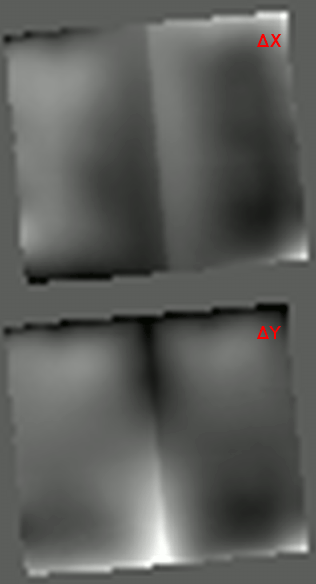
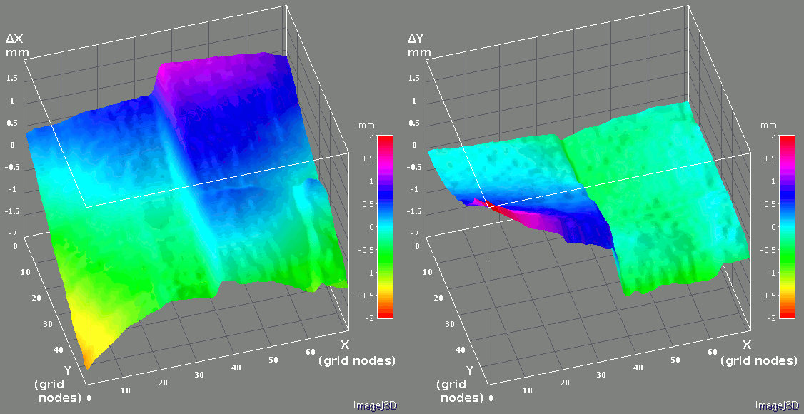
Fig. 6a Pattern grid correction. Combined from the individual measurements shown on Fig. 5a-5b. Full scale is +/- 2mm
Re-running LMA showed some improvement so I repeated the grid re-calculation followed by LMA several times until the decrement in the calculated root mean square of the residual vector fell below the specified threshold – it took about 10 iterations to achieve this.
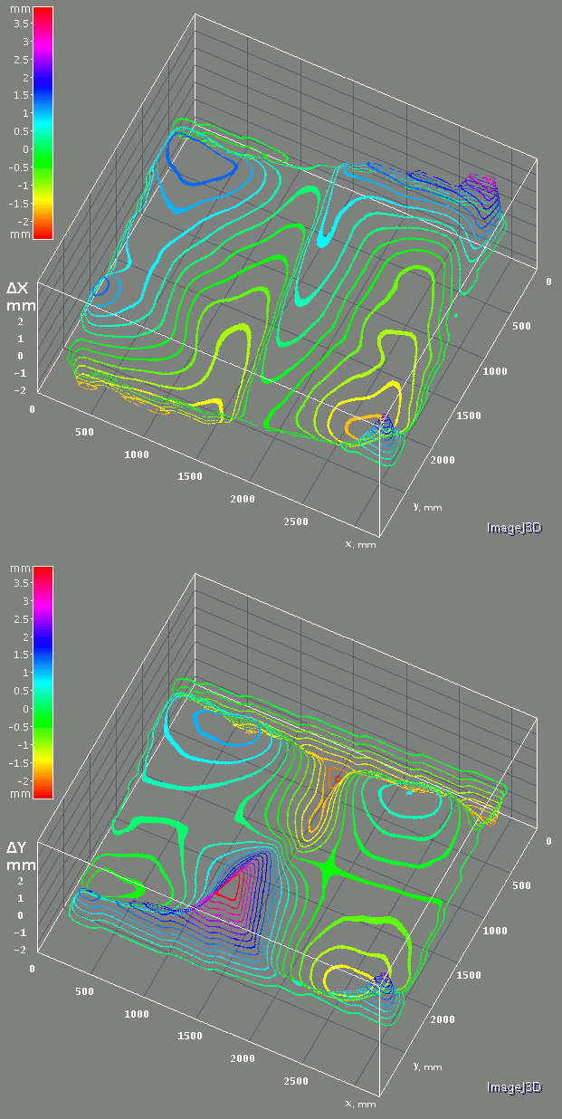
Fig. 6c Reprojection errors after fitting camera extrinsic parameters and intrinsic ones assuming polynomial radial distortions, combined from the individual measurements shown on Fig. 5a-5b. Alternating X and Y differences.
Simultaneously with reducing the RMS of the residual vector this procedure made all the seams caused by overlapping of individual images to fade out and the pattern grid coordinate array converged to the one shown on Fig. 6a-6c.
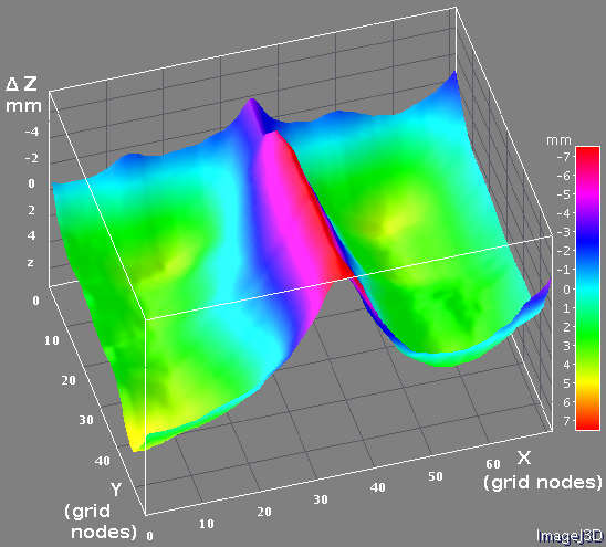
Fig. 6a and Fig. 6b represent the combined pattern grid corrections similarly to the Fig. 5a and Fig. 5b for the partial grid images – the first one with the alternating horizontal and vertical corrections, the second combines both directions as a pseudo-color image. Fig. 6c shows the alternating images of the pattern grid correction as 3d plots.
Coordinate correction, applied to the pattern grid reduced the root mean square of the residual vector from 0.35 to 0.14 pixels and made possible to come back to the measuring the lens distortions.
Measuring and compensating the residual lens distortion
As the grid correction converged to an array and at the same time the radial distortion parameters adjusted by the LMA also reached their final values, I mapped the residual differences of the pattern grid node locations acquired from the set of images to the sensor coordinates, fixed relative to the lens.
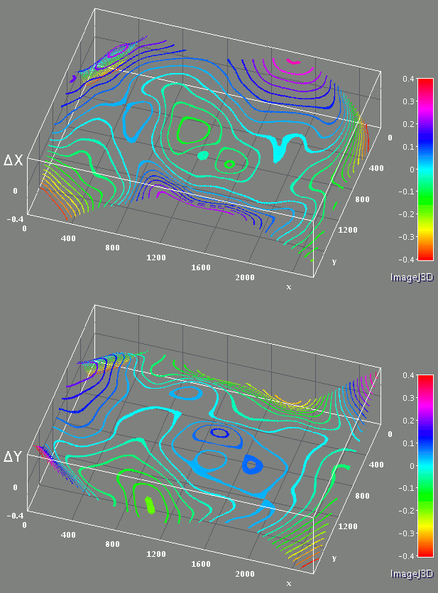
Fig. 7 Residual lens correction after the radial distortion model, alternating for X and Y directions
That allowed me to combine such data from multiple images and measure the difference between the radial lens distortion model used with the registered pattern. Similarly as I did when combining the grid corrections, the program calculated per-image weight functions and then combined the residuals from the 15 images.
When I applied the additional lens correction to each image, I had to freeze the lens distortion coefficients used by the LMA as it could become unstable because the correction array could be calculated for any combination of radial distortion parameters. The averaged correction additionally reduced the RMS of the residual vector to 0.075 pixels. Repetition of the grid correction, LMA (with fixed radial distortion parameters) and calculation of the additional lens correction was stable for the set of the images, but the result did not improve much and the final RMS for the set of images reached 0.069 pixels for the set of 15 images.
This final distortion correction applied “on top” of the radial distortion correction is shown in the last column of Fig. 8, the RMS indicated (0.14px) refers to the correction amount. The same final correction is also shown on Fig. 7 as alternating X and Y corrections, in pixels.
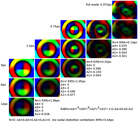
Fig. 8 Residual lens distortion, measured by combining individual images and compensating for the pattern grid errors. The columns correspond to different degrees of polynomials of the radial distortion model, rows show the same residual with the different scale
In addition to applying correction to the lens radial distortion model after all the camera parameters were determined for the best fit, I measured the required correction after the radial polynomial model with reduced number of terms. That helped me to find out how much these terms add to the precision of the model for the particular type of lens that we are using in Eyesis cameras, what is the optimal number of polynomial coefficients in our case.
The results of this comparison are shown in columns of the Fig. 8 where rows show the same functions with different full scale – from 0.375 pixels in the top to 12 pixels in the bottom row. No radial distortion (pinhole camera model) required additional correction with RMS=3.44 pix, single term (Rd/Rs term proportional to radius) reduced RMS to 1.96 pix, two terms – to 1.05 pix and the third term (commonly used, i.e. in Hugin/Panotools ) reduced RMS in our case four times – down to 0.25 pix.
Adding one more term reduced the residual correction, but at this step the image almost lost the prominent so far radial structure, so just adding more terms to the radial polynomial would not help improve the approximation result.
Measuring the 3D locations of the pattern grid nodes
So far I used a two-dimensional model of the pattern grid even as I could see that the pattern on the wall was not flat – there is a rather thick plate that connects two halves of the pattern, same with the reinforcement near the top and wall molding near the floor. The calibration machine will rotate the camera around the center of it’s optical head so most of the camera lenses (but the two specifically designed for distance measurements) will see the pattern with very little parallax and the 5-10mm non-flatness would not lead to significant errors (camera will be located 6 meters from the target pattern).
On the other hand, as there is still a long way ahead before we’ll be able to create 3d models of the nice scenery of the Southern Utah, I was tempted to do a simple 3-d reconstruction of the pattern. And we’ll still need the precise 3-d model for calibration the 2 camera bottom lenses located 1 meter below the rest 24 ones.
For that purpose I added more captured images to the initial set, this time some were acquired from the tripod located some 0.8m to the left of the initial center location, and some – to the right, the total number of simultaneously processed images was 32.
Next was to modify the grid correction procedure to work with 3 coordinates while each image provided only two. And I was looking to the robust method that can still work for the original set of images that were acquired approximately from the same point and it will not try to move the points far in the Z direction.
The first simple modification of the 2-d target grid correction algorithm was to make each image to “vote” for the correction not in the target XY plane, but rather in the direction perpendicular to the line connecting the center of the lens with the grid point being corrected, minimal distance correction that for each camera is equivalent to the required one. Working with the set containing images from multiple points, the result correction will reduce the error in Z direction , but do it at much slower rate than calculated precisely. This method added just a few lines in the code and is still used as a fall-back, in the case of the small parallax of the images resulting in small determinant of the matrix that provided the direct calculation of the correction. That second method was minimizing the sum of squared distances from the corrected 3-d location to the lines connecting each lens location with the 2-d point on the target plane that each camera was voting for.
Both methods were followed by the normalization of the correction to reduce dependence between the effects of the correcting the grid node coordinates and moving the camera. Corrections in X and Y directions have their average values subtracted from each point, correction in Z direction is additionally compensated for tilt, equivalent to rotation of the whole pattern around vertical and horizontal axes.
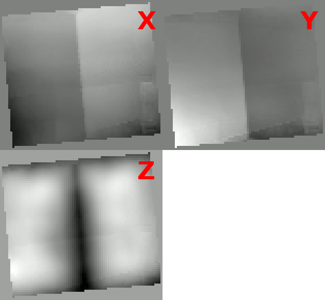
When the 3-d correction was applied, most of the pattern grid differences between the final grid points coordinates and the initial ideal pattern (with equally spaced nodes located on the Z=0 plane) were in the Z direction. That means that the plastic sheets on which the pattern is printed are more bended than stretched. This “redistribution” of the difference from the X and Y to Z direction is visible when comparing Fig. 6a-c and Fig. 9a-c. Large part of the residual errors in X and Y directions is caused by the mismatch of the otherwise uniform pattern halves – shift reveals itself as a step between the halves, rotation – as a different tilt of the halves on both X and Y differences graphs.
It was not so easy to independently verify the measured shape of the pattern, we plan to do more measurements later, so I only measured a single profile in the center of the pattern. For that I used a laser beam parallel to the pattern surface and marked the spots on paper touching the pattern at different locations along the middle horizontal line. The precision of such quick test was about 1 mm and it did match the data from the cross section of Fig. 9c.
One more experiment: camera location from the images
While for the camera calibration we are mostly interested in measuring the mapping from the pixels acquired by the camera at known location to the lines lines in space, I made a separate reverse experiment to test the measurements. That was similar to a rather common task – finding the camera location in space from the available image. Contrary to usual setups where the camera distortion or even lens focal length are either completely unknown or known only approximately, and the shape of the captured objects has to be guessed, in our case the visible object (the pattern grid) was precisely measured and the camera lens was calibrated for distortions – first using the radial distortion model and then additional non-radial correction was applied.
During previous measurements the model was constrained as much as possible, not only the camera intrinsic parameters and the fixed distances and angles in the kinematic model of the camera (including the tripod) were set to be common for all the images, but the location of the tripod as a whole was set not to change for the images belonging to the same group (center, right, left). Program calculated unknown parameters of the model as well as the coordinates of the pattern grid locations while these constrains were imposed.
| Center | Right | Left | |
|---|---|---|---|
| Number of Images | 13 | 6 | 13 |
| X position (mm) | -22.55 | 854.00 | -675.39 |
| Y position (mm) | 67.83 | 64.10 | 64.89 |
| Z position (mm) | 2322.57 | 2361.53 | 2448.79 |
| X std. dev. (mm) | 0.62 | 0.46 | 0.62 |
| Y std. dev. (mm) | 0.57 | 0.51 | 0.52 |
| Z std. dev. (mm) | 0.21 | 0.33 | 0.42 |
| Full std. dev. (mm) | 0.87 | 0.76 | 0.91 |
Then I reran the fitting program while “freezing” the camera intrinsic parameters and the pattern grid correction, but allowing LMA to adjust each of the 3 coordinates of the tripod position and 3 angles defining camera orientation (2 that were actually changed in the tripod head and additional camera roll) for each of the 32 images independently. That means that each (calibrated) camera location was determined by a single image.
Ideally the results of these calculations should be that the tripod position would be exactly the same for all the images of the same group, but there is some discrepancy between these coordinates. The Table 1 summarizes these results, each column average and standard deviation are calculated from the corresponding subset of the images. “Full” standard deviation in the last row is calculated as a square root of the sum of squared deviations in each of the 3 orthogonal directions.
The uncertainty of the camera location along the Z axis is smaller than in X and Y directions, because camera movement along the axis causes more apparent changes in the registered image than when camera is moved perpendicular to the axis (and simultaneously rotating so the optical axis crosses the target plane at the same point.
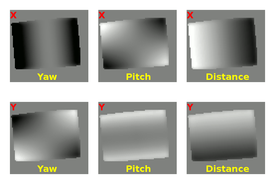
This can be demonstrated if we consider partial derivatives of the pixel coordinates with respect to the two rotations of the camera around the fixed point on the target (that corresponds to X and Y movements) and movement to/from the camera (Z-axis). This derivatives for the center image are shown on the Fig. 10 a,b. The calculated average absolute value (rms) of the reprojection error for horizontal rotation (yaw) around the vertical axis on the target is 6.2 pix/degree, rotation around horizontal axis – 4.0 pix/degree (smaller as the camera is in landscape mode) and moving camera along the Z-axis would cause average error of 0.36pix/mm. Substituting distance to the camera (2322 mm) that results in the following average errors (per mm): X – 0.15 pix/mm, Y- 0.1 pix/mm and Z (unchanged) – 0.36 mm. Multiplying these values by the measured standard deviations in the Table 1. column for the center images result in X – 0.093 pix, Y – 0.057 pix and Z – 0.076 pix – registration precision in pixels needed to provide the measured variations in the camera coordinates.
Results
When we’ll use the calibration machine to calibrate the cameras, both the location of the machine reference point and the coordinates of the pattern grid points will be already known – they can be measured from larger number of evenly overlapping images, and the distance from the camera to the target will be almost 3 times larger than now, so the angular errors caused by linear uncertainty will be proportionally smaller. According to the results of simultaneous fitting of the camera parameters and the target pattern geometrical properties, it will be possible to make angular measurements in the camera field of view with the precision of better than 0.2 pixels over the camera field of view – current constrained fitting of 32 images provided root mean square of combined X and Y mismatch on the sensor of 0.14 pixels (or 0.1 pixels in each direction). With the sensor 2.2 μm pixel period and 4.45 mm focal length, 1 pixel corresponds to 1.7 angular minutes, so 0.2 pixels correspond to 0.35′ angle.
Precision of measurements of the angles between the features in the real-life images will be limited by other factors – registration of the features that have to have enough pixels and high spatial frequency components. The precise calculation of the camera motion using the logged IMU data to compensate for the rolling shutter effect is also the project to be completed, but at least this stage – static pixel mapping of the individual camera is working and provides data to combine the mapping of the sub-cameras into the combined camera and still keep the mapping precision in sub-pixel range. We will work on minimizing the accumulation of the angular errors during “stitching” of the individual pixel maps (in each camera orientation the current pattern wills visible as 10% of the sensor area) by using the precise rotation data and possibly adding additional targets in some other directions – at shorter range but covering larger angle.
All the software described in this post is written in Java as a plugin for ImageJ and is available on our Sourceforge project page under GNU GPLv3 license.


Is this code something wrong?
In this file “csconvert18.v”,at the line 592 and 593,there is the
same code
line592: cbcrmult1 <= sel_cbcrmult1?y[7:0]:pdc[7:0];
line593: cbcrmult1 <= sel_cbcrmult1?y[7:0]:pdc[7:0];
why?
Thank you. Yes, it seems to be a bug – duplicated line. But I believe it was optimized during synthesis and did not influence the result bitstream.
Andrey
whether can the clarity of the image around the central part be increased without regard to lens aberration or flat_lens module function?
Hi Hellomcu,
I’m sorry – I do not understand the question. Can you please clarify it?
Andrey